Week 3 — Reasoning, Judgment & Decision-Making第3週 — 推論・判断・意思決定

Day 1: May 12 (Tue) · Day 2: May 14 (Thu), 2026第1日: 5月12日（火）・第2日: 5月14日（木）, 2026年

Prof. Joseph Austerweilオウステウェイル　ジョセフ教授

Day 1 — The Normative Ideal第1日 — 規範的理想

Tuesday May 12. Day-flow note: tutorial-bracketed lecture. Ira leads opener if Joe is late. Lecture block anchors the EMA / ε-greedy material the tutorial needs to consolidate.

Day 1 Agenda第1日 アジェンダ

• Tutorial Part 1 — Beliefs → Actionsチュートリアル Part 1 — 信念から行動へ 0:00
• Tutorial Part 3 — Reading Code with AIチュートリアル Part 3 — AIとコードを読む 0:15
• Break休憩 0:35
• From Beliefs to Decisions信念から意思決定へ 0:40
• Bayesian Reasoningベイズ的推論 0:45
• Decision Theory意思決定理論 1:05
• The Normative-Descriptive Gap規範と記述のギャップ 1:30
• Break休憩 1:35
• Tutorial Part 2 — EMA vs Bayesianチュートリアル Part 2 — EMA対ベイズ 1:45
• Tutorial Part 4 — MP2 Demoチュートリアル Part 4 — MP2デモ 2:00
• MP2 Launch + Close課題開始 + クロージング 2:10

Today’s downloads本日のダウンロード

From the course page → Phase 2 cards → click and enter the password:

Item	Password
T2 — bridge tutorial	jellyfish-29
MP2 (Assignment) — buggy ε-greedy agent	anglerfish-56

Grab both now so you’re ready when each segment starts.

Course page: aps-i.chibatech.dev/course/

コースページ → Phase 2 のカード → クリックしてパスワードを入力：

項目	パスワード
T2 — ブリッジ・チュートリアル	jellyfish-29
MP2（課題） — バグ入りε-greedyエージェント	anglerfish-56

各セグメントが始まる前に両方ダウンロードしておくこと。

コースページ：aps-i.chibatech.dev/course/

~1 min. Read both passwords aloud — students often miss the dash. Stay on this slide while everyone confirms the downloads started; the tutorial document is inside the T2 zip (bridge-tutorial.md) and the MP2 assignment package includes the buggy code + write-up template. MP2 solution is held back — students get it after MP2 is due.

Tutorial Part 1 — Beliefs → Actionsチュートリアル Part 1 — 信念から行動へ

15 min. Ira leads if Joe is late, otherwise Joe.

Segment shape: - Slide 1 (~7 min): “How did you decide in MP1?” — open discussion. Capture 2-3 student strategies on the board. - Slide 2 (~7 min): “Quick scenario — what would YOU do?” — pose a specific scenario, force commitment, surface the explore-exploit tension. - ~1 min buffer for transition into Tutorial Part 3.

Goal: give Joe (returning from his commute) raw material to call back to in Segment 4 — student names + their proposed strategies on the board. The lecture becomes much more engaging if Joe can say “ proposed always-pick-the-best — let’s see why that’s incomplete.”

Core principle: DO NOT pre-teach formal terms. No “expected utility,” no “ε-greedy,” no “explore-exploit dilemma.” Students should propose these ideas in their own words; Joe gives them the names later. Each slide’s notes have specific don’t-say lists.

If you (Ira) realize partway through that students aren’t engaging: - Skip the discussion format and use the vote-then-defend protocol on slide 2’s notes (3 options, show of hands, ask defenders to explain). - The energy from forcing commitment usually re-engages the room.

How did you decide in MP1?MP1ではどう決めましたか？

You ended MP1 with a recommendation: “Fish in Zone X.”

How did you actually make that decision? What did you do with your beliefs?

Common moves (capture on board):

   • Pick the zone with the highest expected density

   • Weight by confidence — “I’m more sure about Southern Reef”

   • Rule out anything below a survival threshold

We’ll formalize this after the break.

MP1の最後に、皆さんは「ゾーンXで釣る」という判断を出しました。

実際にはどうやってその判断を下しましたか？信念をどう使いましたか？

よくある選び方（黒板に書き留めて）：

   • 期待値が一番高いゾーンを選ぶ

   • 自信の高さで重みづけ — 「Southern Reefは確信がある」

   • 生存に必要な最低ライン未満は除外する

休憩後に [JA-TODO: “formalize” technical term] 形式化します。

Goal: surface 2-3 student decision strategies, capture them on the board, and resist the urge to label them with their formal names. Joe’s lecture (Segment 4) will do that — your job is to give him material to call back to.

Likely student responses + how to push each one:

• “Pick the zone with the highest expected fish.” → Push: “What if your belief about that zone came from one really lucky day? Would you still pick it?” (gets students toward the idea that confidence matters)
• “Pick the zone you’re most confident about.” → Push: “What if you’re very confident in a mediocre zone — would you still pick it?” (gets toward EU vs. risk)
• “Pick the zone where the worst case is still good enough.” → Push: “So you’re using a kind of safety threshold? Tell me more about that.” (gets toward risk-of-ruin)
• Something off-script → Capture it as a 4th option on the board, even if you’re not sure what to do with it. Joe will see it after the break.

If discussion stalls (no one speaks for ~30s): - Read the three bulleted “common moves” out loud as suggestions — “Some people pick the highest-expected zone, some weight by confidence, some rule out below-survival options. Did any of you do something like one of these?” - Once one student speaks, others usually follow.

Don’t say: “That’s expected utility” / “That’s risk-aversion” / any formal term. The lecture introduces those names.

Time: ~5 min discussion + 2 min capture. Move on at 7 min even if discussion has more energy — the next slide (scenario) needs time too.

Quick scenario — what would YOU do?考えてみよう — あなたならどうする？

Your agent has fished 20 times. Current beliefs:

   • Southern Reef: ~60 fish (10 visits, confident)

   • Eastern Shallows: ~55 fish (8 visits)

   • Deep Water: caught 30 fish (only 2 visits — could really be anywhere)

Should the agent ever try Deep Water again? Why or why not?

(Discussion. Capture proposals. We’ll see one formal answer in the lecture block.)

エージェントは20回釣りをした。現在の信念：

   • Southern Reef：約60匹（10回訪問、自信あり）

   • Eastern Shallows：約55匹（8回訪問）

   • Deep Water：30匹獲れた（2回しか訪問していない — 本当はどこにあってもおかしくない）

エージェントはDeep Waterをもう一度試すべきか？なぜ？

（議論。提案を記録。授業では一つの形式的な答えを見ます。）

Goal: surface the explore-vs-exploit tension without naming it. Students should argue about whether it’s worth trying Deep Water (low data, one observation in the empty mode). Joe’s Segment 4 will name this dilemma and introduce ε-greedy.

Setup before posing the question: - Note the asymmetry: Southern Reef has 10 visits and a confident high belief (~60). Deep Water has 2 visits and one mediocre observation (30 fish). The belief about Deep Water is unreliable — recall MP1 said Deep Water is bimodal (could be ~25 or ~85). One observation of 30 doesn’t tell you which mode. - Don’t lead with the asymmetry or the bimodality — pose the question first, then let students notice it themselves. If no one notices in 30s, prompt: “Does the number of visits matter here? What did MP1 say about Deep Water specifically?”

Likely student responses + how to push each one:

• “Fish Southern Reef — it has the highest confident belief.” → Push: “You’ve fished Southern Reef 10 times. What’s the upside of going back vs. trying Deep Water one more time?” (gets toward information gain)
• “Try Deep Water — we don’t know which mode it’s in.” → Push: “So you’d take a worse-looking action right now? Why? What do you get out of it?” (gets toward “value of information” without naming it; rewards students who remember the bimodality)
• “It depends on how many days you have left.” → Excellent. Push: “Say! If you have 100 days left vs. 2 days left, does it change?” (gets toward exploration discount over horizon)
• “Flip a coin.” → Don’t dismiss. Push: “What’s the appeal of randomness here?” (this is literally ε-greedy — capture verbatim)
• “It depends on how risky you are.” → Capture and don’t push (risk attitudes are Segment 4 too).

If discussion stalls: - Pre-write 3 options on the board and ask students to vote: (a) always Southern Reef, (b) try Deep Water one more time, (c) flip a coin between them. Vote count + show of hands. Then ask one volunteer per camp to defend their pick. - The vote-then-defend structure forces commitment and breaks silence.

Don’t say: “This is the explore-exploit dilemma” / “That’s ε-greedy” / “value of information” / any formal term.

Capture for Joe: Write the 2-3 strategies students proposed on the board with the proposing student’s name (or initials, if anonymity is preferred — “A says always Eastern; B says try Western once; C says flip a coin”). Joe references these by name in Segment 4, and that recognition is a strong engagement moment for the named student.

Time: ~7-8 min total. Don’t extend past 10 min even if the discussion is hot — there’s a break coming and students need it.

Up next — Day 1 agenda次はここ — 第1日 アジェンダ

• Tutorial Part 1 — Beliefs → Actionsチュートリアル Part 1 — 信念から行動へ 0:00
• Tutorial Part 3 — Reading Code with AIチュートリアル Part 3 — AIとコードを読む 0:15
• Break休憩 0:35
• From Beliefs to Decisions信念から意思決定へ 0:40
• Bayesian Reasoningベイズ的推論 0:45
• Decision Theory意思決定理論 1:05
• The Normative-Descriptive Gap規範と記述のギャップ 1:30
• Break休憩 1:35
• Tutorial Part 2 — EMA vs Bayesianチュートリアル Part 2 — EMA対ベイズ 1:45
• Tutorial Part 4 — MP2 Demoチュートリアル Part 4 — MP2デモ 2:00
• MP2 Launch + Close課題開始 + クロージング 2:10

Tutorial Part 3 — Reading Code with AIチュートリアル Part 3 — AIとコードを読む

20 min total. Two-stage scaffolded exercise: - Stage 1 (5 min): trace the update formula with AI as calculator. Students discover by computation that old + α · obs diverges and old + α · (obs − old) converges. - Stage 2 (5 min): find the other 2 bugs (Number.MIN_VALUE, off-by-one — both are JS gotchas AI catches easily). - Reveal + discussion (10 min).

Ira-leadable. The two-stage design replaces the original “catch bug 3 from MP1 intuition alone” — students two weeks out from MP1 won’t have that intuition active. Stage 1 gives them a reference point empirically.

The buggy snippetバグのあるコード片

Work with AI. There are 3 bugs. We’ll do this in two stages.

function pickBestZone(beliefs) {
  let bestZone = null;
  let bestValue = Number.MIN_VALUE;
  for (let i = 0; i <= beliefs.length; i++) {
    if (beliefs[i].value > bestValue) {
      bestValue = beliefs[i].value;
      bestZone = beliefs[i];
    }
  }
  return bestZone;
}

function updateBelief(oldBelief, newObs, learningRate) {
  return oldBelief + learningRate * newObs;
}

You don’t need to know JavaScript. You need to know what this code SHOULD do — from MP1.

AIと作業。バグは3つある。2段階で進める。

function pickBestZone(beliefs) {
  let bestZone = null;
  let bestValue = Number.MIN_VALUE;
  for (let i = 0; i <= beliefs.length; i++) {
    if (beliefs[i].value > bestValue) {
      bestValue = beliefs[i].value;
      bestZone = beliefs[i];
    }
  }
  return bestZone;
}

function updateBelief(oldBelief, newObs, learningRate) {
  return oldBelief + learningRate * newObs;
}

JavaScriptの知識は不要。コードが本来何をすべきか — MP1で学んだこと — を理解していればよい。

Display on projector. Two-stage exercise: (1) trace the updateBelief formula with AI as a calculator — see slide 9; (2) then hunt for all 3 bugs, slide 10.

Stage 1 — Trace with AIステージ1 — AIと一緒にたどる

5 minutes. Tutorial → Part 3 → Stage 1.

Trace two candidate updateBelief formulas with AI as a calculator — step by step.

Don’t ask AI which formula is correct yet — that’s your job to figure out from the numbers.

5分。チュートリアル → Part 3 → ステージ1。

updateBeliefの2つの候補式をAIを計算機として使ってたどる — 1ステップずつ。

どちらが正しいかはまだAIに聞かない — それはあなたが数値から判断する。

The full instructions, scenario, and expected step-by-step values live in the tutorial doc — students work from their laptops, not the projector. This slide is just the announce-and-time-box. Expected outcome: students discover empirically that formula (A) old + α · obs diverges past 60 while formula (B) old + α · (obs − old) converges toward 60.

If a student finishes early: have them write down (in one sentence) why formula (A) diverges. Don’t pose any α-edge-case questions — that signals where to look in MP2. The MP2 α bug should be a gacha; students who catch it on their own demonstrate conceptual verification of AI output.

Stage 2 — Find all 3 bugsステージ2 — 3つのバグを全部見つける

5 more minutes. Tutorial → Part 3 → Stage 2.

Stage 1 told you which updateBelief formula is broken. Now find the other 2 bugs — with AI’s help.

Bugs 1 and 2 are JavaScript-level — AI catches them easily.

さらに5分。チュートリアル → Part 3 → ステージ2。

ステージ1でupdateBelief式のどちらが壊れているかは分かった。次は、スニペット内の他の2つのバグを見つける — AIと一緒に。

バグ1と2はJavaScriptレベル — AIが簡単に見つける。

Tutorial doc has the recommended AI prompts. The 5 minutes here is mostly about practicing the AI-collaboration question style. Reveal at the next slide.

Bug revealバグの解答

Bug 1 — Number.MIN_VALUE (JS gotcha — AI catches easily)

MIN_VALUE is the smallest positive number, not −∞. Should be -Infinity.

Bug 2 — i <= beliefs.length (off-by-one — AI catches easily)

Arrays are 0-indexed. Should be i < beliefs.length.

Bug 3 — wrong EMA formula (the conceptual one)

Current: oldBelief + α · newObs

Correct: oldBelief + α · (newObs − oldBelief)

The current formula doesn’t subtract the old belief — beliefs grow without bound.

You catch this with MP1 intuition: beliefs should converge toward truth, not blow up.

バグ1 — Number.MIN_VALUE (JSの落とし穴 — AIが簡単に見つける)

MIN_VALUEは最小の正の数で、−∞ではない。-Infinityが正しい。

バグ2 — i <= beliefs.length (off-by-one — AIが簡単に見つける)

配列は0始まり。i < beliefs.lengthが正しい。

バグ3 — EMA式が誤り (概念的なバグ)

現状: oldBelief + α · newObs

正しい: oldBelief + α · (newObs − oldBelief)

現状の式は古い信念を引いていない — 信念が際限なく増えてしまう。

MP1の直感で気づける：信念は真実にJA-TODO: “converge”収束すべきで、爆発してはいけない。

Bug 3 is the punchline. Frame it: “AI may miss this. You catch it because you understand what learning should look like — that’s the MP2 skill.” Tease the lecture: “The correct formula on the board is what Joe derives in the next block.”

Break — 5 minutes休憩 — 5分

Hard 5 min. Joe should be back by now if late.

Up next — Day 1 agenda次はここ — 第1日 アジェンダ

• Tutorial Part 1 — Beliefs → Actionsチュートリアル Part 1 — 信念から行動へ 0:00
• Tutorial Part 3 — Reading Code with AIチュートリアル Part 3 — AIとコードを読む 0:15
• Break休憩 0:35
• From Beliefs to Decisions信念から意思決定へ 0:40
• Bayesian Reasoningベイズ的推論 0:45
• Decision Theory意思決定理論 1:05
• The Normative-Descriptive Gap規範と記述のギャップ 1:30
• Break休憩 1:35
• Tutorial Part 2 — EMA vs Bayesianチュートリアル Part 2 — EMA対ベイズ 1:45
• Tutorial Part 4 — MP2 Demoチュートリアル Part 4 — MP2デモ 2:00
• MP2 Launch + Close課題開始 + クロージング 2:10

From Beliefs to Decisions信念から意思決定へ

5 min bridge into the formal lecture. Reconnect to Week 2 Chibany + the tutorial work students just did.

Bridge into the lecture授業ブロックへの橋渡し

You just spent 35 minutes connecting MP1 to a buggy agent.

Two weeks ago: you formed beliefs about fish populations.

You ended MP1 with: “Fish in Zone X.”

This week: we formalize what you DO with beliefs.

   • Day 1 — How agents SHOULD reason and decide (normative)

   • Day 2 — How humans ACTUALLY reason and decide (descriptive)

The gap between the two is the intellectual heart of the week.

皆さんは35分かけて、MP1とバグだらけのエージェントを繋げてきた。

2週間前：魚の数についての信念を形成した。

MP1の最後は「ゾーンXで釣る」という結論だった。

今週：信念をどう使うかを形式化する。

   • 第1日 — エージェントはどう推論・決定すべきか（規範的）

   • 第2日 — 人間は実際にどう推論・決定するか（記述的）

両者のギャップが今週の知的な核心。

This is Segment 2 in the new ordering. Anchor: students just experienced the EMA-formula bug. Tee up the lecture as “now let’s name what you almost-saw.”

Up next — Day 1 agenda次はここ — 第1日 アジェンダ

• Tutorial Part 1 — Beliefs → Actionsチュートリアル Part 1 — 信念から行動へ 0:00
• Tutorial Part 3 — Reading Code with AIチュートリアル Part 3 — AIとコードを読む 0:15
• Break休憩 0:35
• From Beliefs to Decisions信念から意思決定へ 0:40
• Bayesian Reasoningベイズ的推論 0:45
• Decision Theory意思決定理論 1:05
• The Normative-Descriptive Gap規範と記述のギャップ 1:30
• Break休憩 1:35
• Tutorial Part 2 — EMA vs Bayesianチュートリアル Part 2 — EMA対ベイズ 1:45
• Tutorial Part 4 — MP2 Demoチュートリアル Part 4 — MP2デモ 2:00
• MP2 Launch + Close課題開始 + クロージング 2:10

Bayesian Reasoning — The Normative Idealベイズ的推論 — 規範的理想

20 min. Quick review (3 min) + Dutch book (5 min, concrete example) + generative model (5 min) + base-rate neglect (4 min) + 3 min buffer. Bayes’ rule should feel like formalization, not first exposure — students saw it in Week 2 + the H&ML elective.

Bayes’ rule — quick reviewベイズの定理 — 復習

In Week 2 you re-derived multiply-and-normalize with Chibany.

P(H \mid D) = \frac{P(D \mid H)\;P(H)}{P(D)} \;\propto\; P(D \mid H)\;P(H)

   • P(H) — prior

   • P(D \mid H) — likelihood

   • P(H \mid D) — posterior

You used this all of MP1. Today we make it rigorous: why Bayes?

(Color convention: orange = prior, blue = likelihood, yellow = posterior. We’ll reuse these later.)

第2週でチバニーを使って掛けて正規化を再導出した。

P(H \mid D) = \frac{P(D \mid H)\;P(H)}{P(D)} \;\propto\; P(D \mid H)\;P(H)

   • P(H) — 事前確率

   • P(D \mid H) — 尤度

   • P(H \mid D) — 事後確率

MP1全体で使ってきた。今日は厳密に：なぜベイズか？

（色の決まり：オレンジ＝事前、青＝尤度、黄色＝事後。後でもう一度使う。）

3 min only. Notation lock-in matches probintro / Chibany. If a student asks “isn’t this what we just did?” — yes, exactly. Today’s new content is the justification, not the rule.

Color convention is established here and reused on the taxicab slide later in this segment. The purpose: when students see the base-rate-neglect example, the colored numbers make “you forgot the orange piece” visually obvious.

Why Bayes? The Dutch bookなぜベイズか — ダッチブック論証

Setup. A forecaster says: P(rain) = 0.6 and P(no rain) = 0.6. The two add to 1.2 — not coherent.

The con. I sell them both tickets at fair-by-their-numbers prices:

• They pay me: $0.60 + $0.60 = $1.20
• Tomorrow, exactly one ticket pays out: $1.00
• I keep $0.20. Guaranteed. No matter what the weather does.

That’s a Dutch book — a set of bets you’re guaranteed to lose.

The generalization. The same logic extends to updating: any belief revision that isn’t Bayes’ rule can be Dutch-booked across two days.

Bayes isn’t one option among many. It’s the unique coherent answer.

設定。ある天気予報士：P(雨) = 0.6、P(雨でない) = 0.6。合計1.2 — 整合的でない。

仕掛け。両方のチケットを彼の言い値で売る：

• 受け取り：$0.60 + $0.60 = $1.20
• 翌日、ちょうど1枚だけ当たる：$1.00
• 純利益$0.20。確実に。天気がどうであれ。

これがダッチブック — 確実に負ける賭けの組み合わせ。

一般化。同じ論理は更新にも当てはまる：ベイズの定理以外の更新規則は、2日間でダッチブックの餌食になる。

ベイズは数ある選択肢の一つではない。唯一の整合的な答え。

~5 min (down from 8 — the concrete example is more efficient than the abstract version). Walk students through the arithmetic: 0.60 + 0.60 = 1.20 in, 1.00 out, 0.20 kept. Pause on “no matter what the weather does” — that’s the punchline.

Once the static axiom-violation case lands, hand-wave the dynamic version: “the same logic with bets across two days shows that ANY update rule other than Bayes’ lets a clever bookmaker extract guaranteed money. We won’t derive it, but the structure is the same — pricing inconsistencies that compound across rounds.” Don’t show the math.

Optional callback if a student pushes: “this is why the prior + likelihood structure has to multiply (not add, not average). Multiplication is the unique operation that makes the axioms hold.”

Time freed (~3 min) can flow into the EMA worked example earlier in the segment, or stay as buffer for questions.

Generative model — think forward生成モデル — 前向きに考える

To use Bayes, ask: “How would the data have been generated if H were true?” Story: a deep-ocean zone is either rich (~80 fish) or empty (~10 fish); observations are noisy.

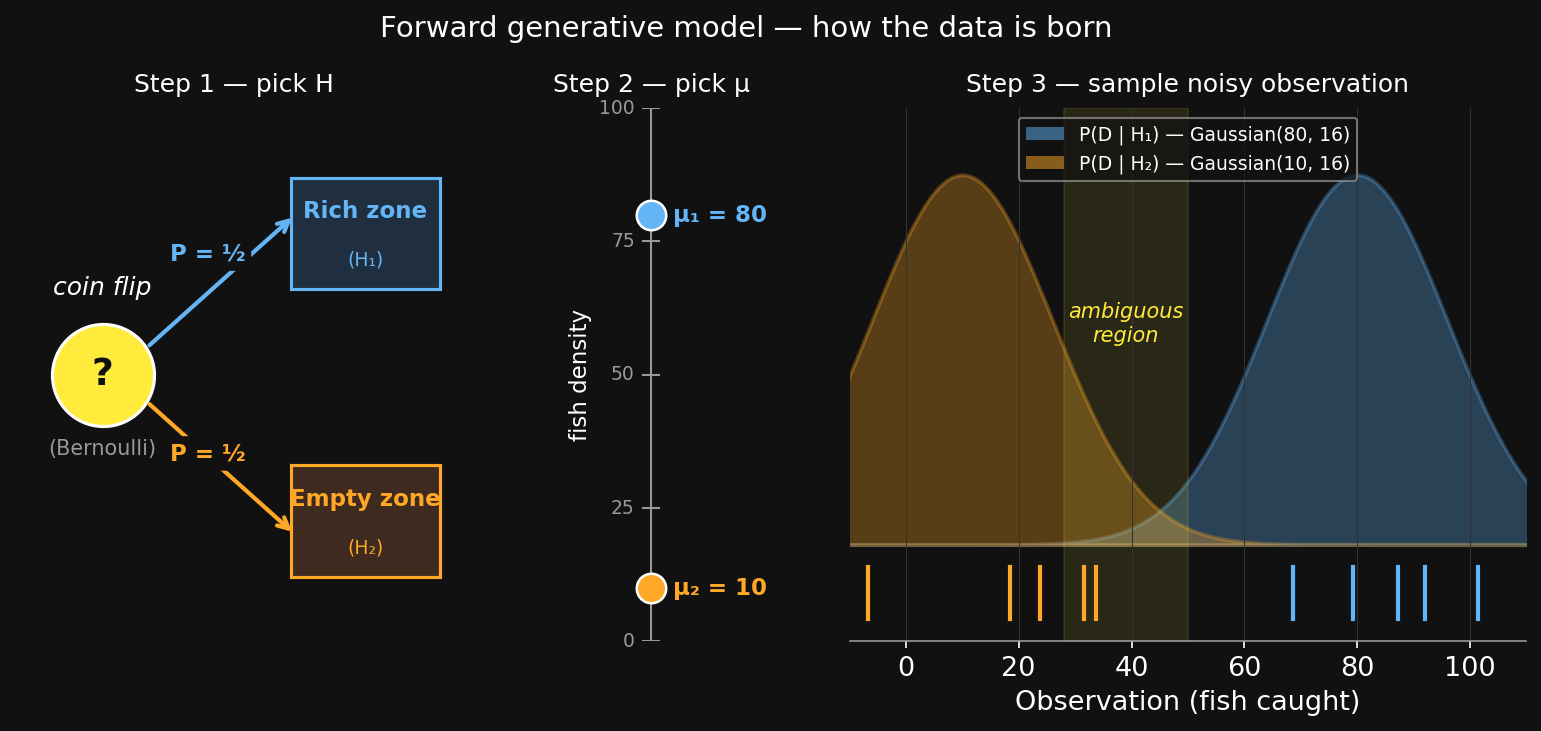
Three steps: flip a coin to pick H (Bernoulli) → that fixes a true mean μ → sample a noisy observation (Gaussian around μ).

ベイズを使うには、こう問う：「仮説Hが真なら、データはどう生成されるか？」 お話：深海ゾーンは「豊富（~80匹）」か「空（~10匹）」、観測にはノイズが乗る。

3つのステップ：コインを投げて H を選ぶ (ベルヌーイ) → 真の平均 μ が決まる → μ の周りでノイズ付き観測 (μ周りのガウス)。

~3 min. Walk through the three panels left to right.

1. Coin flip: which kind of zone? Two equally-likely outcomes. The formal name is “Bernoulli” — flag it but don’t dwell.

2. Picked H fixes μ: rich zone → 80, empty zone → 10. The hypothesis IS the mean.

3. Observations are noisy around μ. Show the two Gaussians and the ambiguous region (~30-50) where an observation could plausibly come from either hypothesis. The 5 sample ticks under each curve illustrate that observations don’t always land near the mean — that’s why we need inference.

The forward direction (this slide) is easy: pick H, draw an observation. The backward direction (next slide) is harder: given an observation, which H?

This binary case is a simplification. MP1 had 20 hypotheses, not 2 — but the structure is identical: pick a hypothesis, sample a noisy observation. Inference works the same way no matter how many hypotheses you have.

Bayesian inference — invert the arrowベイズ推論 — 矢印を逆向きに

The generative model goes forward:

   H → D   (pick a zone, then sample fish)

Bayesian inference goes backward:

   D → H   (saw an observation; which zone produced it?)

Example: you observe 40 fish.

   • Under H₁ (rich, μ=80): an obs of 40 is unusual but possible.

   • Under H₂ (empty, μ=10): an obs of 40 is also unusual but possible.

   • Bayes weighs both → posterior over H.

The forward model gives you P(D \mid H). The backward inversion is what students computed in MP1 — multiply by the prior, normalize, get P(H \mid D).

生成モデルは前向き：

   H → D   （ゾーンを選び、魚を観測）

ベイズ推論は逆向き：

   D → H   （観測値があった。どのゾーンから生成された？）

例：40匹を観測した。

   • H₁（豊富、μ=80）の下では：40は珍しいが起こりうる。

   • H₂（空、μ=10）の下でも：40は珍しいが起こりうる。

   • ベイズは両方を重みづけ → Hの事後分布。

前向きモデルからP(D \mid H)。逆向きの反転がMP1でやったこと — 事前分布を掛けて正規化、P(H \mid D)を得る。

~2 min. The inversion is the point of Bayesian inference — given that data was generated by some unknown H, what’s our best guess about H?

For obs=40, we’re squarely in the ambiguous region from the previous slide. Both hypotheses give it nontrivial likelihood. The prior + Bayes’ rule resolves the tie. With a uniform prior, the posterior split would tilt slightly toward H₂ (because 40 is closer to 10 than to 80 in std-units: |40-10|/12 ≈ 2.5σ vs |40-80|/12 ≈ 3.3σ → H₂ is more likely).

If a sharp student asks “what about MP1’s 20 hypotheses?” — same idea, just over more H. The forward model is “pick a density bin, sample a Gaussian observation around the bin center”; the backward inversion is what their update() function did. The simulation in MP1 explicitly did this — point at the code if there’s time.

This is the practical insight that makes Bayes usable, not just a formula. Forward = generative. Backward = inference.

Base-rate neglect基準率の無視

Taxicab problem (Tversky & Kahneman, 1972):

Hit-and-run. 85% of cabs are Green, 15% Blue. A witness identifies the cab as Blue and is correct 80% of the time.

Gut answer: P(Blue | witness) ≈ 0.80.   Most people stop here.

Bayes:

P(\text{Blue} \mid W) \;=\; \frac{P(W \mid \text{Blue})\;P(\text{Blue})}{P(W \mid \text{Blue})\,P(\text{Blue}) + P(W \mid \text{Green})\,P(\text{Green})}

\frac{\textcolor{#64B5F6}{0.80}\cdot\textcolor{#FFA726}{0.15}}{\textcolor{#64B5F6}{0.80}\cdot\textcolor{#FFA726}{0.15} + \textcolor{#64B5F6}{0.20}\cdot\textcolor{#FFA726}{0.85}} \;=\; \textcolor{#FFEB3B}{0.41}

You forgot the prior — that most (85%) of the cabs are Green. The base rate matters as much as the witness reliability.

MP1: a strong prior + one noisy observation barely moved the posterior.

タクシー問題（Tversky & Kahneman, 1972）：

ひき逃げ事件。タクシーの85%が緑、15%が青。目撃者は青と特定し、正解率は80%。

直感的な答え：P(青 | 目撃) ≈ 0.80。   多くの人はここで止まる。

ベイズ：

P(\text{青} \mid W) \;=\; \frac{P(W \mid \text{青})\;P(\text{青})}{P(W \mid \text{青})\,P(\text{青}) + P(W \mid \text{緑})\,P(\text{緑})}

\frac{\textcolor{#64B5F6}{0.80}\cdot\textcolor{#FFA726}{0.15}}{\textcolor{#64B5F6}{0.80}\cdot\textcolor{#FFA726}{0.15} + \textcolor{#64B5F6}{0.20}\cdot\textcolor{#FFA726}{0.85}} \;=\; \textcolor{#FFEB3B}{0.41}

事前確率を忘れていた — そもそも85%のタクシーは緑。基準率は目撃者の信頼性と同じくらい重要。

MP1で経験：強い事前 + 1つのノイズ観測では事後はほとんど動かない。

4 min. Students saw this in the H&ML elective — refresh, not first exposure.

Color reuse from the Bayes’ rule slide: orange = prior, blue = likelihood, yellow = posterior. Color-coding is quiet visual aid only — the punchline names the concept (prior, base rate) rather than the color, to avoid confusion with the cab-color hypotheses (Green/Blue).

Walk through the equation: numerator is “likelihood × prior” — the joint probability of (Blue cab AND witness says Blue). Denominator is the marginal — total probability of “witness says Blue” across both hypotheses. Result: 0.12 / 0.29 = 0.41.

The deeper lesson — students should leave with: when the prior is strongly against H, you need very strong evidence (high likelihood ratio) to overcome it. The witness has likelihood ratio 4:1 (0.80/0.20), but the prior is 1:5.67 (0.15/0.85), so the posterior odds are 4:5.67 ≈ 1:1.4 → P(Blue) ≈ 0.41.

Connection to MP1: same structure plays out when a student’s “Southern Reef: 40-60” prior was strong and one observation came in at 78. The posterior barely moved because likelihood × prior gave little weight to the new value.

Day 2 picks this up under “heuristics and biases.”

Up next — Day 1 agenda次はここ — 第1日 アジェンダ

• Tutorial Part 1 — Beliefs → Actionsチュートリアル Part 1 — 信念から行動へ 0:00
• Tutorial Part 3 — Reading Code with AIチュートリアル Part 3 — AIとコードを読む 0:15
• Break休憩 0:35
• From Beliefs to Decisions信念から意思決定へ 0:40
• Bayesian Reasoningベイズ的推論 0:45
• Decision Theory意思決定理論 1:05
• The Normative-Descriptive Gap規範と記述のギャップ 1:30
• Break休憩 1:35
• Tutorial Part 2 — EMA vs Bayesianチュートリアル Part 2 — EMA対ベイズ 1:45
• Tutorial Part 4 — MP2 Demoチュートリアル Part 4 — MP2デモ 2:00
• MP2 Launch + Close課題開始 + クロージング 2:10

Decision Theory — What Should You Do?意思決定理論 — 何をすべきか？

25 min. Beliefs → decisions. Callbacks: (a) Tutorial Part 1 student proposals for the 20-fish scenario, (b) Tutorial Part 3 Bug 3 as the negative example for the EMA derivation.

Pacing note for EU subsegment (5 slides): Action vs outcome → expected value → “not all fish equal” → utility function → expected utility formalization. Each slide is one conceptual move. If running short on time, slides 22a (action vs outcome) and 22b (expected value with explicit table) can be condensed verbally; slides 22c–22e (utility function and EU formula) are the conceptual core that should not be rushed.

Narrative thread: all examples in this segment use MP1’s canonical 5 zones (refresher slide next). Southern Reef = reliable baseline; Deep Water = bimodal high-variance. The contrast carries through EU → risk → explore-exploit → ε-greedy.

Refresher — the 5 fishing zones from MP1復習 — MP1の5つの釣りゾーン

zone	prior description	character
Southern Reef	“40-60, reliable”	steady baseline
Eastern Shallows	“50-70, recent activity”	moderately known
Western Bay	“could be anything”	wide-open prior
Kelp Forest	“20-40, recovering”	outdated prior
Deep Water	“sometimes huge (75-95), sometimes empty (15-40)”	bimodal, unpredictable

We’ll use these names throughout today. Watch for Southern Reef (reliable) vs Deep Water (high-variance) — that contrast carries the rest of Day 1.

ゾーン	事前情報	性質
Southern Reef（南の珊瑚礁）	「40-60、安定」	安定したベースライン
Eastern Shallows（東の浅瀬）	「50-70、最近活動あり」	やや既知
Western Bay（西の湾）	「なんとも言えない」	幅広い事前
Kelp Forest（藻場）	「20-40、回復中」	古い事前情報
Deep Water（深海）	「巨大（75-95）か空（15-40）の二極」	二峰性、予測困難

今日の例ではこれらの名前を一貫して使う。Southern Reef（安定）と Deep Water（高分散）の対比が本日後半を貫く。

~1-2 min refresher. The point is not to re-teach the zones, just to surface them so subsequent slides can use the names without explanation. Students saw all 5 in MP1.

The Southern Reef vs Deep Water contrast is the spine of the segment: - EU: Southern Reef has reliable EV; Deep Water has same EV with high variance. - Risk: Southern Reef clears the survival threshold reliably; Deep Water fails sometimes. - Explore-exploit: Southern Reef is well-known; Deep Water has a bimodal prior so each observation is highly informative. - ε-greedy: exploit Southern Reef, explore Deep Water.

If a student asks why MP1 priors said “20-40” for Kelp Forest but actual was 50-65 — say “good catch, that’s a teaching point about outdated priors. Today we’re using the priors as given.” Don’t rabbit-hole.

Note on Deep Water bimodality: this came up in MP1 class — students wished they’d been told the bimodal structure earlier. Day 1 explicitly gives them the bimodal prior here so they can see why it matters for ε-greedy.

Beliefs are not decisions信念は決定ではない

You have posteriors for each zone.

Where do you fish?

A decision rule maps beliefs → actions.

Today: four decision-theoretic concepts you’ll use in MP2:

   • Expected utility

   • Risk attitudes

   • Explore-exploit + ε-greedy

   • EMA as a simplified update

各ゾーンの事後分布はある。

どこで釣る？

決定規則は信念 → 行動の写像。

今日扱うのはMP2で使う4つの概念：

   • 期待効用

   • リスク態度

   • 探索-搾取と ε-greedy

   • 簡易更新としてのEMA

Open Segment 4. Reference the Tutorial Part 1 student proposals on the board (“you said exploit-the-best, you said weight-by-confidence — let’s name those”).

Action vs outcome行動と結果

You fish Southern Reef for 5 days. Catches: 60, 50, 70, 40, 55.

   • Action: fish in Southern Reef — same every day.

   • Outcome: 60, 50, 70, 40, 55 — different every day.

Same action, different outcomes. Why? The world is noisy.

Average over 5 days: 55. Pretty good — but no single day was exactly 55.

Southern Reefで5日間釣りをした。漁獲：60, 50, 70, 40, 55。

   • 行動：Southern Reefで釣る — 毎日同じ。

   • 結果：60, 50, 70, 40, 55 — 毎日違う。

同じ行動、違う結果。なぜ？世界はノイズが乗るから。

5日間の平均：55。まあまあ良い — でもどの日もちょうど55ではなかった。

~2 min. The action vs. outcome distinction is foundational for the rest of decision theory and is often where students stumble. Action = what you do (one choice). Outcome = what happens (varies due to world noise). Make sure students hear this distinction clearly before moving on.

The “no day was exactly 55” line previews the gap between EV and any individual outcome — relevant for the risk slide later.

Expected value — what to expect on average期待値 — 平均して何を予想するか

5 days isn’t much data. With more data, the average stabilizes. The limit is the expected value.

Suppose Southern Reef’s true outcome distribution is:

outcome (fish)	probability
40	10%
50	30%
60	40%
70	20%

Expected fish per day:

E[\text{fish}] = 0.10 \cdot 40 + 0.30 \cdot 50 + 0.40 \cdot 60 + 0.20 \cdot 70 = 57

Each outcome weighted by how often it happens. That’s all “expected” means.

5日間のデータは少ない。データが増えれば平均は安定する。その極限が期待値。

Southern Reefの真の結果分布が次の通りだったとする：

結果（魚）	確率
40	10%
50	30%
60	40%
70	20%

1日あたりの期待漁獲量：

E[\text{魚}] = 0.10 \cdot 40 + 0.30 \cdot 50 + 0.40 \cdot 60 + 0.20 \cdot 70 = 57

各結果をそれがどれだけ頻繁に起こるかで重みづけ。それだけ。

~2 min. Walk through the arithmetic on the board — students should see the weighted-sum operation explicitly with concrete numbers BEFORE they see Σ notation. “0.10 times 40, plus 0.30 times 50, …” is the same operation as the Σ formula they’ll see in slide 22d.

If a sharp student asks “where do those probabilities come from?” — say “the same way MP1’s beliefs came from observations. With enough fishing days, you’d estimate them empirically. We’re skipping that step here.”

Don’t introduce u(·) yet. Right now we’re still counting fish, not valuing them.

Not all fish are equal魚はみな同じではない

Counting fish breaks down when fish are worth different amounts.

Japanese market values (rough wholesale): Tuna ~¥10,000/fish, Sardine ~¥100/fish — a 100× gap.

Two zones, two strategies (on a good day for each):

zone	catches per day	total daily value
Southern Reef (sardine school)	50 sardines	50 × ¥100 = ¥5,000
Deep Water (good day — high mode)	27 sardines + 3 tuna	27·¥100 + 3·¥10,000 = ¥32,700

Deep Water on a good day catches fewer fish but earns 6× more.

Counting fish ≠ measuring goodness. We need a function that turns an outcome into a value-to-you.

魚に価値の違いがあると、ただ数えるだけでは足りない。

日本市場の概算卸売価格： マグロ 1匹 約¥10,000、イワシ 1匹 約¥100 — 100倍の差。

2つのゾーン、2つの戦略（各ゾーンの良い日）：

ゾーン	1日の漁獲	1日の総価値
Southern Reef（イワシの群れ）	イワシ50匹	50 × ¥100 = ¥5,000
Deep Water（良い日 — 高い側）	イワシ27匹 + マグロ3匹	27·¥100 + 3·¥10,000 = ¥32,700

Deep Waterの良い日は、魚の数は少ないが、収入は6倍。

魚の数を数えるだけでは「良さ」は測れない。結果を「自分にとっての価値」に変換する関数が必要。

~2 min. The Southern Reef vs. Deep Water contrast is the punchline: Deep Water (on a good day) has fewer total fish but is much more valuable. Students should immediately see why “average fish caught” misses the point.

This motivates the utility function. The next slide names it.

Optional aside if a student goes deep: real bluefin tuna at Toyosu auction can clear ¥1,000,000 for a prized individual fish. ¥10,000 is the “ordinary tuna” wholesale ballpark. Sardine retail varies seasonally but ¥100/fish is a reasonable midpoint. Numbers are illustrative — they’re in the right ballpark but not commodity-trading precise.

The utility function効用関数

A utility function u(\cdot) takes an outcome and returns a number that reflects how much you care. Per fish: u(\text{sardine}) = 100, u(\text{tuna}) = 10{,}000.

Total utility of an outcome o (a bag of fish) — sum the per-fish utilities:

U(o) \;=\; \sum_{f \in o} u(f)

   • Southern Reef: U(50\text{ sardines}) = 50 \cdot 100 = \mathbf{5{,}000}

   • Deep Water: U(27\text{ sardines} + 3\text{ tuna}) = 27 \cdot 100 + 3 \cdot 10{,}000 = \mathbf{32{,}700}

Compare U, not raw counts. An aquarium with u(\text{tuna}) = 0 would prefer Southern Reef — different u, different best zone.

効用関数u(\cdot)は、結果を「自分にとってどれだけ良いか」の数値に変換する関数。1匹あたり：u(\text{イワシ}) = 100、u(\text{マグロ}) = 10{,}000。

結果o（魚の袋）の合計効用 — 1匹ずつの効用を合計：

U(o) \;=\; \sum_{f \in o} u(f)

   • Southern Reef：U(\text{イワシ50匹}) = 50 \cdot 100 = \mathbf{5{,}000}

   • Deep Water：U(\text{イワシ27匹} + \text{マグロ3匹}) = 27 \cdot 100 + 3 \cdot 10{,}000 = \mathbf{32{,}700}

比べるのはU、漁獲数ではない。 水族館がu(\text{マグロ})=0ならSouthern Reefが最良 — uが変われば最良ゾーンも変わる。

~3 min. Two-tier notation: - u(\cdot) — per-fish utility, evaluated on a single fish. - U(\cdot) — total utility of an outcome (a multiset of fish), defined as the sum of per-fish utilities.

This separation matters because (a) it makes the math precise — “u = 50 \cdot 100” was sloppy because u is a function, not a number; the value of u(\text{sardine}) is 100, and the total over 50 sardines is the sum, naturally written as U. And (b) it sets up the Σ structure students will see again on the next-next slide for expected utility: EU(a) = \sum_i p_i \cdot U(o_i). Lower-case u for atoms, capital U for outcomes; same shape (a sum) at both levels.

The aquarium aside (“they value tuna at ¥0”) is now a cleaner concept: same outcomes, same U(o) structure, but a different per-fish u(\cdot) — specifically u(\text{tuna}) = 0. That difference at the per-fish level changes which outcome has higher U.

If you have time, ask: “What’s an outcome where YOUR utility wouldn’t be linear in fish count?” → diminishing marginal utility (Day-2 Bernoulli concept).

EU in action — should you buy a lottery ticket?EU実演 — 宝くじを買うべきか？

Setup: A ticket costs ¥100. 5% chance to win ¥5,000.

Two outcomes (relative to your wallet):

   • Lose: −¥100 with probability 0.95

   • Win: +¥4,900 (¥5,000 prize − ¥100 ticket) with probability 0.05

Expected utility:

E[U] = 0.95 \cdot (-100) + 0.05 \cdot (4{,}900) = -95 + 245 = \mathbf{+150}

Positive EU. By the rule, you should buy. (Though only by ¥150 — small expected gain.)

Most real lotteries: realistic prize-and-probability structures give negative EU. Don’t buy those.

設定：チケット¥100。5%の確率で¥5,000当選。

2つの結果（財布から見て）：

   • ハズレ：−¥100、確率0.95

   • 当選：+¥4,900（¥5,000賞金 − ¥100チケット）、確率0.05

期待効用：

E[U] = 0.95 \cdot (-100) + 0.05 \cdot (4{,}900) = -95 + 245 = \mathbf{+150}

EUは正。ルールに従えば買うべき。（ただし¥150だけ — 期待利益は小さい。）

現実の宝くじ：実際の賞金と確率の構造は負のEUを与えることが多い。それは買わない。

~2 min. The lottery example is from Joe’s PSYC414 Lec 12. It’s a clean two-outcome EU calculation that students can do in their heads — no village context, no fish, just probability × utility.

Why it’s useful here: gives students one concrete, single-number EU computation BEFORE the Σ formula. The 22e formula then becomes “the same operation, generalized to many outcomes.” Without this slide, students see Σ for the first time on 22e and may bounce off.

Practical aside: this lottery has positive EU, but realistic lotteries (state lotteries, scratch tickets) almost always have negative EU once probabilities are accurate. PSYC414 Lec 12 has a 7-row payoff table demonstrating this — could pull it up if students are interested.

Numerically: if a student questions “but it’s only +150 — is that really worth it?” the answer is YES under EU theory; risk-neutral agents take any positive-EU bet. But the next slide (village starving) shows when risk attitudes override EU. Frame this slide as “EU says yes, but only barely.” Sets up the pivot.

Expected utility — putting it together期待効用 — まとめ

For each action a with outcomes o_i (bags of fish) and probabilities p_i:

EU(a) = \sum_i p_i \cdot U(o_i) \;\;\;\text{where}\;\;\; U(o_i) = \sum_{f \in o_i} u(f)

Decision rule: pick the action with the highest EU.

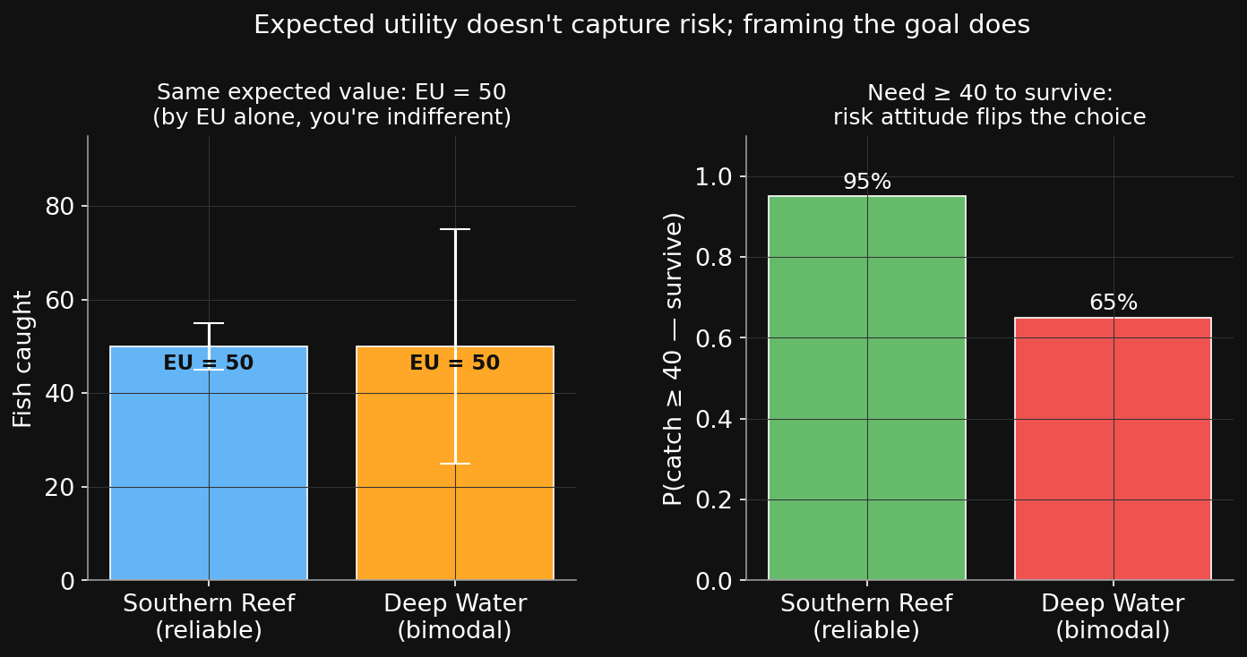
But: EU alone misses something. Suppose the village needs ¥3,000/day to eat tonight.

   • Southern Reef: guarantees ¥5,000. Eats every day.

   • Deep Water: 50/50 between ¥0 and ¥10,000 (bimodal). Same EU = ¥5,000.

   • On Deep Water’s bad day → ¥0. Empty stomachs tonight.

Are you still indifferent?

各行動a、結果o_i（魚の袋）、確率p_iについて：

EU(a) = \sum_i p_i \cdot U(o_i) \;\;\;\text{ただし}\;\;\; U(o_i) = \sum_{f \in o_i} u(f)

決定規則：期待効用が最大の行動を選ぶ。

しかし：EUだけでは足りない。村は今晩食べるのに1日¥3,000必要だとしよう。

   • Southern Reef：¥5,000確実。毎日食べられる。

   • Deep Water：¥0と¥10,000の半々（二峰性）。EUは同じ¥5,000。

   • Deep Waterの悪い日 → ¥0。今晩は空腹。

それでもまだ無差別？

~2 min. Now the formula is just naming what we already did. Σ = “sum over outcomes.” u(oᵢ) = “value of outcome i.” pᵢ = “probability of outcome i.” Each piece has been seen.

The starvation framing motivates the next slide: when survival depends on a threshold (here, ¥3,000 to eat), variance becomes critical. EU treats the two zones as equivalent; survival doesn’t. Make the consequence of variance vivid — people go hungry, not “you might feel bad about losing.”

The next slide formalizes this with P(survive) — same data, framed as probability of clearing the survival threshold. That visualizes the same insight quantitatively.

If students balked at Σ earlier in the course, this is your chance to name it as “the same weighted-sum we’ve been doing.” It’s an abbreviation, not new math.

Risk: when variance mattersリスク：分散が効くとき

Same EU; but if you need ≥ 40 to survive, P(survive) flips the choice. Risk-of-ruin reframe — variance matters when your utility function has a cliff. This is why “expected utility” alone misses something humans naturally feel.

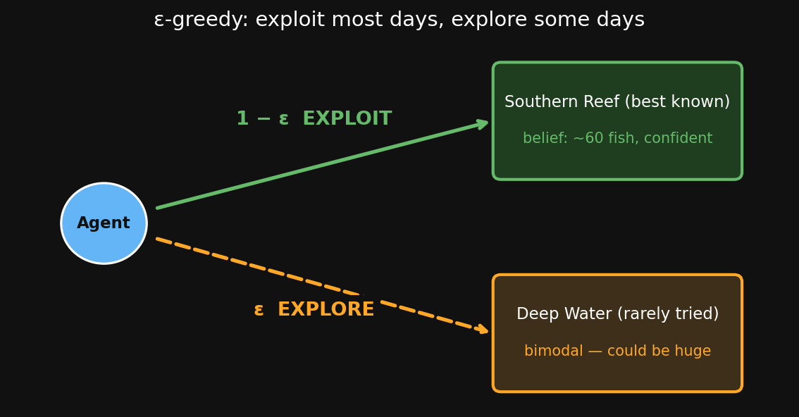
Explore vs exploit探索 vs 搾取

Setup: You’ve fished Southern Reef 10 times (consistent ~60 fish — you’re confident). You’ve fished Deep Water only once and got 30 fish.

Should you try Deep Water again? Not because you think it’s better — but because you don’t yet know which mode it’s in.

Recall: Deep Water’s prior is bimodal — could be ~25 (empty) or ~85 (huge). Your one observation of 30 is consistent with the empty mode… but the huge mode is still on the table.

Exploit = pick the zone you currently believe is best (Southern Reef).

Explore = try a less-known zone to refine your belief (Deep Water).

Your Tutorial Part 1 proposals were exploit-only. The agent needs both.

設定：Southern Reefで10回釣った（一貫して約60匹 — 自信あり）。Deep Waterでは1回だけ釣り、30匹獲れた。

Deep Waterをもう一度試すべきか？「Deep Waterの方が良い」と思うからではなく — まだ二峰性のどちらの側か分からないから。

思い出して：Deep Waterの事前は二峰性 — 約25（空）か約85（巨大）か。1回の観測30は空側と整合的だが、巨大側もまだ排除できない。

搾取（exploit） = 現時点で最良と信じるゾーンを選ぶ（Southern Reef）。

探索（explore） = 情報の少ないゾーンを試して信念を磨く（Deep Water）。

Tutorial Part 1での皆さんの提案は搾取のみだった。エージェントには両方必要。

Direct callback to Tutorial Part 1’s quick-scenario slide. If the board still has student proposals, point at them now.

The bimodal hook is the key teaching moment here. Deep Water’s prior says “either ~25 or ~85” — that’s exactly when one observation is highly informative and exploration has high value. With a unimodal prior, one observation gives you a Gaussian update; with a bimodal prior, one observation can almost-discriminate which mode you’re in. This is what students wished they had been told in MP1; today we’re explicit about it.

If a student asks: “what if my one Deep Water observation had been 85 instead of 30?” — answer: “Then you’d be more confident in the high mode, and you’d actually want to exploit Deep Water, not Southern Reef. But with one observation you’re still uncertain — the next observation matters a lot either way.”

The ε-greedy ruleε-greedyルール

With probability (1−ε) exploit; with probability ε explore randomly. Simple, robust, the workhorse of MP2.

EMA update — what your agent doesEMA更新 — エージェントの動作

Exponential Moving Average:

\text{new} = \text{old} + \alpha \cdot (\text{obs} - \text{old})

Nudge the belief a fraction \alpha of the way toward the new observation.

Convergence: the mean of the belief tracks truth. Step-to-step fluctuations persist — their size is bounded by \alpha \cdot (observation noise).

   • \alpha = 0 — never updates; belief frozen at the prior.

   • \alpha small (e.g. 0.1) — slow but steady; tiny fluctuations once near truth.

   • \alpha moderate (e.g. 0.3) — balanced; converges in ~5–10 steps, then oscillates within a small band.

   • \alpha = 1 — belief = latest observation; no averaging across past obs.

The averaging effect comes from \alpha < 1. Smaller α → smoother but slower; larger α → more responsive but noisier.

指数移動平均（EMA）：

\text{new} = \text{old} + \alpha \cdot (\text{obs} - \text{old})

信念を新しい観測に向かって\alphaの割合だけ近づける。

収束：信念の平均が真値を追跡する。ステップごとの揺らぎは残る — その大きさは \alpha \cdot（観測ノイズ）で有界。

   • \alpha = 0 — 全く更新しない；信念は事前のまま固定。

   • \alpha 小（例：0.1） — 遅いが安定；真値に近づくと揺らぎは微小。

   • \alpha 中（例：0.3） — 均衡；5–10ステップで収束し、真値の周りを小さな幅で振動。

   • \alpha = 1 — 信念 = 直近の観測；過去の観測を平均化しない。

平均化の効果は \alpha < 1 から生まれる。αが小さいほど滑らかだが遅い；大きいほど反応的だがノイジー。

~3 min. The convergence definition is the new key content. Two things students need to leave with:

1. What convergence means for EMA. The mean of the belief tracks truth, but individual updates keep moving. Fluctuations don’t shrink to zero — they shrink to a bounded amplitude proportional to α·noise. (For students who think of stochastic-approximation theory: that’s the decreasing-α setting, where α_t = 1/t. MP2 uses fixed α, so it’s tracking-with-bounded-oscillation, not vanishing-fluctuation. Don’t go into this unless asked.)

2. Where averaging comes from. With α<1, each new estimate is a weighted mix of old + new; α=1 is the upper endpoint where the formula collapses to new = obs. Describe both endpoints (α=0, α=1) symmetrically as degenerate cases. Don’t single out α=1 with stronger emphasis — that tips MP2’s bug. The MP2 bug should be a gacha: students who catch it on their own demonstrate they’re verifying AI output against conceptual understanding; students who don’t will learn from the reveal.

The next slide visualizes all three regimes (α=0.1, 0.3, 1.0) over 30 steps so students can see the bounded-fluctuation story.

Direct callback to Tutorial Part 3 Bug 3. “You knew Bug 3’s formula was wrong from MP1 intuition — now you have the right formula AND the right intuition for α. Both pieces together are how you’ll catch MP2’s bugs.” (Don’t specify which bugs — they’ll discover those.)

Worked example — EMA step by stepワーク例 — EMAを一歩ずつ

Setup: zone with true density 70. Tool noise ≈ 10. Four observations: 65, 72, 68, 74.

EMA rule: \text{new} = \text{old} + \alpha \cdot (\text{obs} - \text{old})    with \alpha = 0.3.    Start at belief = 50 (“I don’t know”).

Step 1. obs = 65.   gap = 65 − 50 = 15.   new = 50 + 0.3 × 15 = 50 + 4.5 = 54.5

Step 2. obs = 72.   gap = 72 − 54.5 = 17.5.   new = 54.5 + 0.3 × 17.5 = 54.5 + 5.25 = 59.75

Step 3. obs = 68.   gap = 68 − 59.75 = 8.25.   new = 59.75 + 0.3 × 8.25 = 59.75 + 2.475 = 62.23

Step 4. obs = 74.   gap = 74 − 62.23 = 11.77.   new = 62.23 + 0.3 × 11.77 = 62.23 + 3.53 = 65.76

Each step: gap × α, then add to old belief. After 4 obs, belief = 65.76. Truth = 70. Still ~4 off.

設定：真の密度70のゾーン。ツールのノイズ ≈ 10。4回の観測：65, 72, 68, 74。

EMAルール： \text{new} = \text{old} + \alpha \cdot (\text{obs} - \text{old})    \alpha = 0.3。   信念 = 50（「分からない」）から開始。

ステップ1。 obs = 65。  ギャップ = 65 − 50 = 15。  new = 50 + 0.3 × 15 = 50 + 4.5 = 54.5

ステップ2。 obs = 72。  ギャップ = 72 − 54.5 = 17.5。  new = 54.5 + 0.3 × 17.5 = 54.5 + 5.25 = 59.75

ステップ3。 obs = 68。  ギャップ = 68 − 59.75 = 8.25。  new = 59.75 + 0.3 × 8.25 = 59.75 + 2.475 = 62.23

ステップ4。 obs = 74。  ギャップ = 74 − 62.23 = 11.77。  new = 62.23 + 0.3 × 11.77 = 62.23 + 3.53 = 65.76

各ステップ：ギャップ × α、それを古い信念に足す。4観測後、信念 = 65.76。真値 = 70。まだ約4ずれている。

~4 min. Walk through this slowly. Students won’t do this arithmetic in their heads — read each step out loud, point at the screen as you compute.

Per-step verbal pattern: - “The gap is observation minus old belief: (obs − old).” - “We move only α of the way, so we multiply that gap by α.” - “Add that to the old belief — that’s the new belief.”

Step 1 example verbal: “We saw 65. Our belief was 50. The gap is 65 minus 50 = 15. We multiply 15 by 0.3 to get 4.5. We add 4.5 to 50 — new belief is 54.5.”

The shape to surface: the gap shrinks as belief approaches truth. Step 1 gap = 15, step 2 gap = 17.5 (the obs was high), step 3 gap = 8.25 (smaller), step 4 gap = 11.77. The update size scales with how surprising the observation was.

Tutorial Part 3 callback: “You traced exactly this kind of step in Tutorial Part 3 Stage 1. The correct formula gave you a converging belief; the buggy formula didn’t.”

On the next slide we’ll compare these EMA numbers to what Bayes would do with the same data.

Same data — Bayes catches up faster同じデータ — ベイズの方が速い

Same 4 observations. Same starting point. Two different methods.

step	obs	EMA belief	Bayes — mean (std)
0	—	50.00	50.00 (28.83)
1	65	54.50	64.99 (9.99)
2	72	59.75	68.50 (7.07)
3	68	62.23	68.33 (5.77)
4	74	65.76	69.75 (5.00)

After 4 obs: EMA = 65.76 (still ~4 off truth 70). Bayes = 69.75 (essentially on truth) — and reports std 28.83 → 5.00.

Bayes is more powerful with an uninformative prior, but EMA is simpler — often good enough. Next: what does an informative prior buy you?

同じ4観測。同じ出発点。2つの異なる手法。

ステップ	観測	EMA信念	ベイズ — 平均 (std)
0	—	50.00	50.00 (28.83)
1	65	54.50	64.99 (9.99)
2	72	59.75	68.50 (7.07)
3	68	62.23	68.33 (5.77)
4	74	65.76	69.75 (5.00)

4観測後：EMA = 65.76（真値70からまだ約4ずれ）。ベイズ = 69.75（ほぼ真値ぴったり） — さらに標準偏差は28.83 → 5.00。

事前分布が無情報のときベイズは強力、EMAはシンプル — 多くの問題で十分。次：情報のある事前分布だとどうなる？

~3 min. Comparison slide. Two takeaways:

1. EMA is slower at chasing truth when starting from an uninformative point. After 4 obs at α=0.3, EMA’s effective memory is ~3-4 obs and each obs is down-weighted. Bayes (with a uniform prior over 20 density bins) treats every observation as equally informative — and the posterior concentrates fast.

2. EMA gives you one number; Bayes gives you a number AND a measure of confidence. By step 4 Bayes is saying “density is 69.75 ± 5”; EMA is saying just “65.76.” If you needed to decide under risk-of-ruin (need ≥ 40 to survive), the std matters.

Don’t let students conclude “Bayes is just better.” MP2 uses EMA precisely because EMA is simpler, cheaper, and good enough when you’re tracking a slowly-changing density without needing confidence. The point is to know the trade-off, not to declare a winner.

Next slide extends this with three Bayesian priors (uniform, good, wrong) to show what an informative prior buys you.

What if the prior IS informative?事前分布がある場合は？

Same observations, same noise. Three priors: Uniform (no info), Good (\mathcal{N}(70, 10)), Wrong (\mathcal{N}(30, 10)).

step	obs	Uniform	Good (μ₀=70)	Wrong (μ₀=30)
0	—	50.00	70.00	30.04
1	65	64.99	67.50	47.50
2	72	68.50	69.00	55.67
3	68	68.33	68.75	58.75
4	74	69.75	69.80	61.80

1. A good prior gets you close from step 0 — but uniform catches up by step 2.

2. A wrong prior is overruled by data — slowly. Still 8 off after 4 obs.

3. Data dominates with enough observations. The prior shapes early steps, not the long run.

同じ観測、同じノイズ。3つの事前分布：一様（情報なし）、良い（\mathcal{N}(70, 10)）、間違い（\mathcal{N}(30, 10)）。

ステップ	観測	一様	良い (μ₀=70)	間違い (μ₀=30)
0	—	50.00	70.00	30.04
1	65	64.99	67.50	47.50
2	72	68.50	69.00	55.67
3	68	68.33	68.75	58.75
4	74	69.75	69.80	61.80

1. 良い事前分布なら最初から真値近く — でも一様もステップ2で追いつく。

2. 間違った事前分布はデータにゆっくり覆される。4観測後でもまだ8ずれている。

3. 観測が十分あればデータが支配する。事前分布は初期を形作るが、長期的には消える。

Story: data eventually wins, but bad priors leave fingerprints. The wrong-prior column climbs from 30 → 47 → 55 → 58 → 62, never catching up to 70 in 4 steps. With 8-10 more observations it would — but in MP2 students don’t get unlimited observations per zone.

Real-world implication for MP2: if your agent’s initial belief in the buggy code is too far from truth, the agent might never visit the zone enough to fix it (it’ll see the low belief and exploit elsewhere). The interaction of belief + decision-rule is where bugs hide.

This slide is also where prospect-theory loss aversion (Day 2) gets foreshadowed — humans are even worse than this Bayesian “wrong prior” agent at letting data overrule beliefs.

EMA convergence — three α, three regimesEMAの収束 — 3つのα、3つの挙動

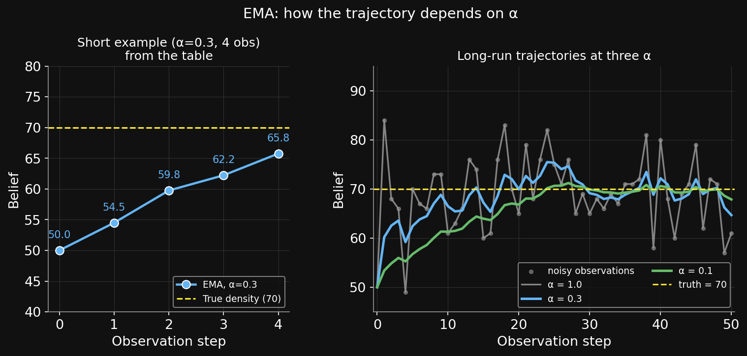
Left: the worked example from the table (α=0.3, 4 obs). Right: 50 noisy observations from the same true density (70), three different α.

   • α=0.1 — slow climb, very small fluctuations near truth

   • α=0.3 — converges quickly, bounded oscillation

   • α=1.0 — belief = latest observation; full noise amplitude

This is what convergence looks like in practice: the mean of the belief tracks truth; the fluctuations shrink to a bounded amplitude that depends on α.

左：表の短い例（α=0.3、4観測）。右：同じ真の密度（70）から50個のノイズ観測、3つの異なるα。

   • α=0.1 — 緩やかに上昇、真値近くでは微小な揺らぎ

   • α=0.3 — 速やかに収束、有界な振動

   • α=1.0 — 信念 = 直近の観測；フルノイズ振幅

実際の収束はこう見える：信念の平均は真値を追跡し、揺らぎはαに応じた有界な振幅まで縮む。

~2-3 min. The figure visualizes the convergence story from the previous slide. Walk through the three lines on the right panel:

• (α=1.0) — point at the jagged line. “If you set α=1, every step is just the latest noisy fish count — the belief mirrors each observation.” Describe neutrally as the upper endpoint of the α spectrum. Don’t label it broken; don’t hint that this matters in MP2. Students who recognize the same pattern in MP2 catch the bug; students who don’t will learn from the reveal — that’s the intended gacha.

• Blue (α=0.3) — point at the steady-but-oscillating line. “This is what convergence looks like. The belief climbs from 50 to ~70 in about 5-10 steps, then oscillates around 70 with small amplitude. The mean is right; there are still fluctuations because each observation is noisy.”

• Green (α=0.1) — point at the slow-climb line. “Smaller α means slower convergence but smaller fluctuations. The agent here is still climbing toward 70 at step 30. Tradeoff: steadier but slower.”

The dotted gray dots are the actual noisy observations the EMA is averaging across. Useful for showing what the agent “sees” each step before averaging.

L1/L2 framing reminder: this is a visualization of EMA’s behavior at different α. The L1/L2 comparison (EMA vs full Bayes for the same problem) was the worked-example slides earlier; this slide is now specifically about EMA’s parameter sensitivity.

Up next — Day 1 agenda次はここ — 第1日 アジェンダ

• Tutorial Part 1 — Beliefs → Actionsチュートリアル Part 1 — 信念から行動へ 0:00
• Tutorial Part 3 — Reading Code with AIチュートリアル Part 3 — AIとコードを読む 0:15
• Break休憩 0:35
• From Beliefs to Decisions信念から意思決定へ 0:40
• Bayesian Reasoningベイズ的推論 0:45
• Decision Theory意思決定理論 1:05
• The Normative-Descriptive Gap規範と記述のギャップ 1:30
• Break休憩 1:35
• Tutorial Part 2 — EMA vs Bayesianチュートリアル Part 2 — EMA対ベイズ 1:45
• Tutorial Part 4 — MP2 Demoチュートリアル Part 4 — MP2デモ 2:00
• MP2 Launch + Close課題開始 + クロージング 2:10

The Normative-Descriptive Gap規範と記述のギャップ

5 min. Tease Day 2.

Humans are not normative agents人間は規範的エージェントではない

Everything I just told you is about how agents SHOULD reason and decide.

But humans DON’T — at least not always.

Day 2 (Thursday):

   • Heuristics and biases (representativeness, confirmation)

   • Prospect theory (framing, loss aversion, probability weighting)

Is the gap a flaw in human cognition, or a feature?

ここまでは、エージェントがどう推論・決定すべきかという話。

しかし人間はそう動かない — 少なくとも常には。

第2日（木曜）：

   • ヒューリスティックとバイアス（代表性、確証バイアス）

   • プロスペクト理論（フレーミング、損失回避、確率重みづけ）

このギャップは認知の欠陥か、機能か？

Closing question is the bridge to Day 2’s central tension.

Break — 10 minutes休憩 — 10分

Hard 10. Long break before the consolidation tutorial — students need it.

Up next — Day 1 agenda次はここ — 第1日 アジェンダ

• Tutorial Part 1 — Beliefs → Actionsチュートリアル Part 1 — 信念から行動へ 0:00
• Tutorial Part 3 — Reading Code with AIチュートリアル Part 3 — AIとコードを読む 0:15
• Break休憩 0:35
• From Beliefs to Decisions信念から意思決定へ 0:40
• Bayesian Reasoningベイズ的推論 0:45
• Decision Theory意思決定理論 1:05
• The Normative-Descriptive Gap規範と記述のギャップ 1:30
• Break休憩 1:35
• Tutorial Part 2 — EMA vs Bayesianチュートリアル Part 2 — EMA対ベイズ 1:45
• Tutorial Part 4 — MP2 Demoチュートリアル Part 4 — MP2デモ 2:00
• MP2 Launch + Close課題開始 + クロージング 2:10

Tutorial Part 2 — EMA vs Bayesian Side-by-Sideチュートリアル Part 2 — EMA vs ベイズ並列比較

15 min. Now lands as consolidation, not first exposure. Joe leads.

Side-by-side並列比較

MP1 (Bayesian):

   • posterior[i] = prior[i] * likelihood[i] (then normalize)

   • Maintains a full distribution (20 bins)

   • Each obs refines the entire shape

MP2 (EMA):

   • new = old + α * (obs − old)

   • One number per zone (point estimate)

   • Each obs nudges the number toward what was observed

Same Marr L1 problem. Different L2 algorithm.

MP1（ベイズ）：

   • posterior[i] = prior[i] * likelihood[i]（その後正規化）

   • 完全な分布を保持（20ビン）

   • 各観測が分布全体を修正

MP2（EMA）：

   • new = old + α * (obs − old)

   • ゾーンごとに1つの数値（点推定）

   • 各観測が観測値の方へ数値を押す

同じMarr L1問題。異なるL2アルゴリズム。

Already lectured. This is consolidation. Frame it as “you saw the formula in the lecture; here’s the comparison to MP1.”

α extremesαの両極

\alpha	new =	what happens
0.0	1.0·old + 0.0·obs	never updates
0.1	0.9·old + 0.1·obs	steady, prior dominates
0.5	0.5·old + 0.5·obs	balanced
1.0	0.0·old + 1.0·obs	only the latest obs

The endpoints are degenerate — α=0 never learns, α=1 forgets everything. Useful α is somewhere in between.

\alpha	new =	起こること
0.0	1.0·old + 0.0·obs	更新なし
0.1	0.9·old + 0.1·obs	安定、事前に支配
0.5	0.5·old + 0.5·obs	均衡
1.0	0.0·old + 1.0·obs	直近の観測のみ

両端は退化している — α=0は学習しない、α=1は過去を忘れる。有用なαはその間。

Treat the table as conceptual context only. Both endpoints get equal weight — α=0 (never updates) and α=1 (only latest obs) are both shown as degenerate; don’t single out α=1 with stronger emphasis. The MP2 α=1.0 bug should be a “gacha” — students who catch it on their own demonstrate that they’re verifying AI solutions against their conceptual understanding. Students who miss it learn the lesson when it’s revealed: AI can produce running code that does the wrong thing.

Don’t say “watch for this in MP2” or “if you see jagged beliefs, look at α.” Those tip the answer. Let the table teach the EMA formula’s parameter space — full stop.

Up next — Day 1 agenda次はここ — 第1日 アジェンダ

• Tutorial Part 1 — Beliefs → Actionsチュートリアル Part 1 — 信念から行動へ 0:00
• Tutorial Part 3 — Reading Code with AIチュートリアル Part 3 — AIとコードを読む 0:15
• Break休憩 0:35
• From Beliefs to Decisions信念から意思決定へ 0:40
• Bayesian Reasoningベイズ的推論 0:45
• Decision Theory意思決定理論 1:05
• The Normative-Descriptive Gap規範と記述のギャップ 1:30
• Break休憩 1:35
• Tutorial Part 2 — EMA vs Bayesianチュートリアル Part 2 — EMA対ベイズ 1:45
• Tutorial Part 4 — MP2 Demoチュートリアル Part 4 — MP2デモ 2:00
• MP2 Launch + Close課題開始 + クロージング 2:10

Tutorial Part 4 — MP2 Demoチュートリアル Part 4 — MP2デモ

10 min. Live demo of the correct MP2 simulation. ε = 0, ε = 1, ε = 0.1. Show belief panel converging.

Live demoライブデモ

Open the correct MP2 simulation in browser.

Three runs to demonstrate:

   • ε = 0 — pure exploit (locks onto first decent zone)

   • ε = 1 — pure explore (random — never settles)

   • ε = 0.1 — balanced (mostly exploits, occasional explore)

Watch the belief panel. Beliefs should converge toward truth over time.

MP2 ships with intentional bugs. Some break this convergence.

ブラウザで正しいMP2シミュレーションを開く。

3つのランを見せる：

   • ε = 0 — 純粋な搾取（最初のまずまずのゾーンに固定）

   • ε = 1 — 純粋な探索（ランダム — 落ち着かない）

   • ε = 0.1 — 均衡（主に搾取、時々探索）

信念パネルを見る。信念は時間と共に真実に収束すべき。

MP2には意図的なバグがある。一部はこの収束を壊す。

Don’t just talk through it — actually run the demo. The convergence visualization is the payoff. Pause and let students watch.

What MP2 looks likeMP2の課題内容

You’ll receive a buggy ε-greedy agent. Some bugs are syntax (AI catches). Some are conceptual — like Tutorial Part 3 Bug 3 — where you need MP1-style understanding.

Your job:

  1. Run the simulation. Observe the agent’s behavior.

  2. Work with AI to read the code and find bugs.

  3. Use MP1 understanding to catch what AI misses.

  4. Document what you found AND how you found it.

Grading emphasizes WHY a bug is wrong, not just spotting it.

バグだらけのε-greedyエージェントを受け取る。構文バグ（AIが見つける）もあれば、Tutorial Part 3 バグ3のような概念的なものもある — そこではMP1的な理解が必要。

やること：

  1. シミュレーションを動かす。エージェントの挙動を観察。

  2. AIと一緒にコードを読み、バグを見つける。

  3. MP1の理解でAIが見落とすバグを捕まえる。

  4. 何を、どうやって見つけたかを記録。

評価は「バグを見つけたか」より「なぜそれがバグか」を重視。

Set expectations. Reduce anxiety. Document-the-process is the assignment, not just bug-count.

Up next — Day 1 agenda次はここ — 第1日 アジェンダ

• Tutorial Part 1 — Beliefs → Actionsチュートリアル Part 1 — 信念から行動へ 0:00
• Tutorial Part 3 — Reading Code with AIチュートリアル Part 3 — AIとコードを読む 0:15
• Break休憩 0:35
• From Beliefs to Decisions信念から意思決定へ 0:40
• Bayesian Reasoningベイズ的推論 0:45
• Decision Theory意思決定理論 1:05
• The Normative-Descriptive Gap規範と記述のギャップ 1:30
• Break休憩 1:35
• Tutorial Part 2 — EMA vs Bayesianチュートリアル Part 2 — EMA対ベイズ 1:45
• Tutorial Part 4 — MP2 Demoチュートリアル Part 4 — MP2デモ 2:00
• MP2 Launch + Close課題開始 + クロージング 2:10

MP2 Launch + CloseMP2始動 + クロージング

40 min MP2 launch + 10 min close. Distribute. First debugging cycle. Circulate — watch for “paste-into-Claude-and-say-fix-this” antipattern; redirect to “run the simulation, observe behavior.”

Day 1 close第1日 クロージング

Thursday: heuristics, biases, and prospect theory.

Is the gap between normative and descriptive a flaw in human cognition, or a feature?

Read for Thursday:

   • Griffiths, Chater, & Tenenbaum — Ch 1 (continued)

   • Wu & Toyokawa — Tutorial 1

Bring MP2 progress notes — we’ll resume debugging discussion.

木曜：ヒューリスティック、バイアス、プロスペクト理論。

規範と記述のギャップは認知の欠陥か、機能か？

木曜までに読むもの：

   • Griffiths, Chater, & Tenenbaum — 第1章（続き）

   • Wu & Toyokawa — チュートリアル1

MP2の進捗メモを持参 — デバッグ議論を再開する。

Day 1 ends here.

Day 2 — The Descriptive Reality第2日 — 記述的な現実

Thursday May 14. Students arrive having done MP2 first cycle. Open with energy — Linda problem if low energy.

Day 2 structure (3 hr total): - 0:00–0:35 — H&B (35 min, expanded: representativeness in hiring + all 3 CRT items) - 0:35–0:55 — Prospect theory (20 min) - 0:55–1:05 — Break (10 min) - 1:05–1:35 — Nudging (30 min, Japan-framed: organ donation, kyūshoku, iDeCo, fishing-policy/MP4 setup) - 1:35–2:28 — MP2 in-class work (53 min, Joe + Ira circulate) - 2:28–2:48 — MP2 guided discussion (20 min, bug-driven group convo) - 2:48–2:56 — Three-week arc + Week 4 preview (8 min) - 2:56–3:00 — Buffer / Q&A

Day 2 Agenda第2日 アジェンダ

• Heuristics and biasesヒューリスティックとバイアス 0:00
• Prospect theoryプロスペクト理論 0:35
• Break休憩 0:55
• Nudging — choice architectureナッジ — 選択アーキテクチャ 1:05
• MP2 in-class workMP2 授業内作業時間 1:35
• MP2 guided discussionMP2 ガイド付き議論 2:28
• Three-week arc + Week 43週間の流れ + 第4週 2:48
• Buffer / Q&A予備 / Q&A 2:56

Why we worked through the mathなぜ数式を一歩ずつ追ったのか

Day 1 was a lot. Bayes. Expected utility. Generative models. EMA. Today is softer — stories, demos, biases you can feel. So why grind through the math?

Without a normative account, there are no biases.

   • “People are bad at probability” → bad compared to what?

   • “People polarize on the same data” → polarized away from what?

   • “People take risks they shouldn’t” → shouldn’t by what standard?

Bayes + EU give us the ruler. Bias must also be systematic — random errors average out; systematic ones predict direction.

Day 1: built the ruler. Day 2: measure the gap. Week 4+ (nudging, MP4): use it to design.

第1日は内容が多かった。ベイズ、期待効用、生成モデル、EMA。今日は柔らかい — 物語、デモ、体感バイアス。ではなぜ数式を追ったのか？

規範的な説明がなければ、バイアスというものは存在しない。

   • 「人は確率が苦手」→ 何と比べて苦手？

   • 「同じデータで人は極化する」→ 何から離れて極化する？

   • 「人はリスクを取りすぎる」→ どの基準で取りすぎ？

ベイズと期待効用がものさしをくれる。さらにバイアスは体系的でなければならない — ランダム誤差は平均で消える、体系的誤差は方向を予測する。

第1日：ものさしを作った。第2日：ズレを測る。第4週以降（ナッジ、MP4）：設計に使う。

~3 min. This is the conceptual hinge for the whole week. It’s worth saying slowly.

Three arguments to make verbally, building on the slide:

1. The asymmetry between Day 1 and Day 2 is real. Day 1 was hard — formal probability theory, derivations, formulas. Day 2 is concrete and visceral — students will experience biases firsthand in the next 35 min via Linda, CRT, etc. The temptation will be to think Day 2 is “the easy day” or “the soft day.” It’s not — it’s the day where Day 1’s framework actually gets applied to the question that matters: are humans like this normative agent? The math wasn’t decoration.

2. “Bias” is a normatively-loaded term. You literally cannot identify a bias without a normative model — otherwise you just have a pattern in behavior. The Tversky/Kahneman program of the 1970s was a theoretical achievement precisely because they used existing normative models (probability, EU) as the diagnostic instrument. Lord/Ross/Lepper’s biased-assimilation result is only a result because Bayes tells us what coherent updating looks like; otherwise it’s “they disagreed about the studies.” With Bayes, it’s “they updated in OPPOSITE directions on the same evidence — which is impossible for any coherent updater.”

3. Systematic vs random matters. This is the deepest point. If bias were random, it would be noise — we’d say “human cognition is noisy” and shrug. The reason H&B is a science is that biases are predictable: same person, same situation, same wrong answer. Predictability requires a model. The normative model lets us see the bias; the descriptive model (heuristics) lets us predict it. Two halves.

4. MP2 callback (verbal, optional): “You spent yesterday afternoon debugging an EMA agent. The ONLY reason you could catch the conceptual bug is that you had Bayes/EU in your head as the benchmark. If you didn’t know what ‘correct learning’ looks like, you couldn’t tell broken from working. The same logic applies to human cognition.”

Set this slide up as a defense of yesterday’s effort. The students did the hard work — give them the payoff explicitly.

Heuristics and biasesヒューリスティックとバイアス

35 min. Major heuristics: representativeness (Linda + dot-com bubble + hiring/tenure), availability, confirmation bias (with Lord/Ross/Lepper polarization + Consider-the-Opposite intervention). Close with System 1 vs System 2 via the full 3-question Cognitive Reflection Test (bat-and-ball + widget machines + lily pad). Most slides are pulled from Joe’s PSYC414 Lec 11–12 framing — concrete real-world examples and live demonstrations carry the pedagogy more than the village/MP2 callbacks. Pacing: if running short, availability is the most omittable; the hiring/tenure slide is also droppable but valuable for grounding representativeness beyond “stock-market silliness.” Everything else lands harder.

Meet Linda — which is more likely?リンダ問題 — どちらが起こりやすい？

Linda is 31, single, outspoken, and very bright. She majored in philosophy. As a student, she was deeply concerned with issues of discrimination and social justice, and also participated in anti-nuclear demonstrations.

Which is more probable?

   A. Linda is a bank teller.

   B. Linda is a bank teller AND active in the feminist movement.

Pick one. Don’t compute — just say which feels more likely.

リンダは31歳、独身、率直で、非常に頭脳明晰。哲学を専攻していた。学生時代は差別や社会正義の問題に深く関わり、反核デモにも参加していた。

どちらの確率が高いと思う？

   A. リンダは銀行員である。

   B. リンダは銀行員であり、かつフェミニスト運動に積極的である。

ひとつ選ぶ。計算するのではなく、どちらがより起こりやすいと感じるかを答える。

~2 min. Live vote — A or B — before revealing the next slide. Don’t say anything about probability theory yet. The goal is to get students to commit publicly to an answer (show of hands) so the next slide’s reveal lands as a contradiction with their own intuition.

Common outcome: 70-90% pick B. Capture the rough split on the board (“13 out of 5 of you said B” — adjusting for class size; with 5 students likely 3-4 will say B).

If a student picks A and is asked why: usually they’ve seen the problem before, OR they’re doing the math in their head. Validate: “right — and we’ll see WHY on the next slide.” Don’t reveal more yet.

Don’t say “conjunction fallacy” or any technical term on this slide. That’s the next slide.

Linda — the set pictureリンダ — 集合の図

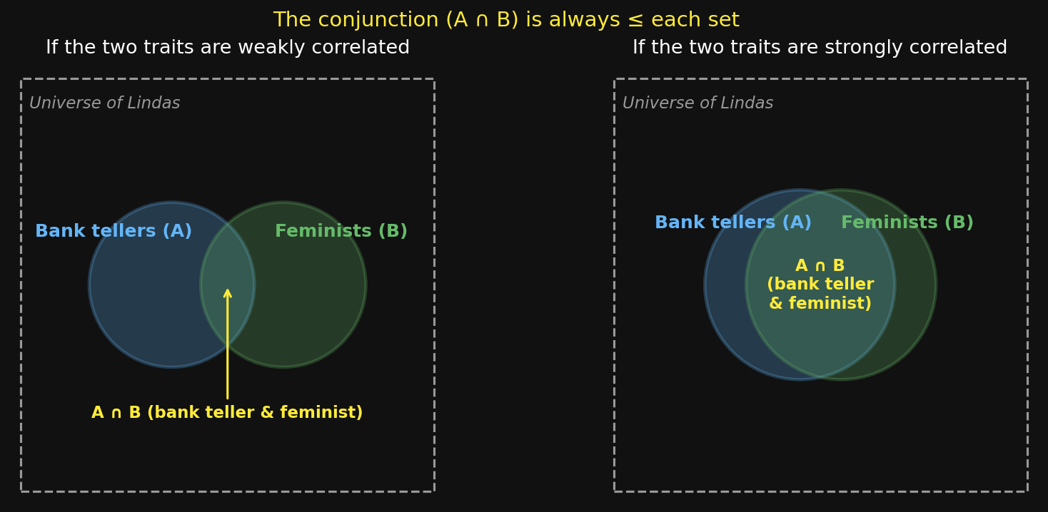
Whatever you believe about how often bank tellers are feminists, the intersection is at most as big as either set. P(A \cap B) \leq P(A), P(A \cap B) \leq P(B).

銀行員とフェミニストの相関について何を信じていても、交わりは各集合より大きくはなれない。 P(A \cap B) \leq P(A)、 P(A \cap B) \leq P(B)。

~1-2 min. Show this before the inequality on the next slide. Walk through:

• “Look at the universe of Lindas. Some are bank tellers (blue); some are feminists (green); some are both (intersection).”
• “Now — does it matter HOW correlated those two traits are? On the left, bank tellers and feminists are mostly different people (weak correlation). On the right, almost every bank teller is also a feminist (strong correlation). Two very different worlds.”
• “In BOTH cases, the intersection — the set of people who are both — is at most as big as either circle. It’s a subset. Geometrically. There’s no way the intersection can be bigger than the part.”
• “So when we ask ‘is Linda more likely to be a bank teller, or both a bank teller AND a feminist?’ — by pure set logic, the AND has to be smaller-or-equal. The answer doesn’t depend on your prior about whether Lindas tend to be feminists.”

This sets up the formal inequality on the next slide as a consequence of the geometric picture rather than as the punchline itself.

Linda — the conjunction fallacyリンダ — 連言の誤謬

Most people pick B. But:

P(\text{bank teller} \cap \text{feminist}) \;\leq\; P(\text{bank teller})

The conjunction can never be more likely than its parts. Every Linda-who-is-feminist-and-bank-teller is also a Linda-who-is-bank-teller. B is a subset of A.

The shortcut: rather than computing probability, we substitute an easier question — “how well does B resemble the stereotype of who Linda is?”

The stereotype-match is high for B (philosophy major, discrimination, anti-nuclear) and low for A (just “bank teller”). So B feels more likely — even though it can’t be.

This is representativeness: judging probability by similarity instead of by the math. Sometimes it works. Here it produces a logical contradiction.

多くの人はBを選ぶ。しかし：

P(\text{銀行員} \cap \text{フェミニスト}) \;\leq\; P(\text{銀行員})

連言（かつ）の確率は、その要素単独の確率を絶対に超えない。リンダが銀行員かつフェミニストなら、必ず銀行員でもある。BはAの部分集合。

ショートカット：確率を計算する代わりに、より簡単な問いに置き換える — 「Bはリンダのステレオタイプにどれだけ似ているか？」

ステレオタイプ一致度は、Bは高い（哲学専攻・差別・反核）、Aは低い（単に「銀行員」）。だからBの方が起こりやすく感じる — 論理的にはあり得ないのに。

これが代表性ヒューリスティック：確率を数学ではなく類似度で判断する。うまくいくこともある。ここでは論理的矛盾を生む。

~3 min. Reveal the answer. The “always” in the inequality is important: it’s not a probabilistic claim that usually P(A∩B) ≤ P(A) — it’s a mathematical certainty. The set of bank-teller-feminists is a subset of the set of bank-tellers.

Framing (from PSYC414): representativeness is substituting an easier question for a hard one. Computing P(L ∩ B) requires probability theory; computing “how Linda-like does she sound?” doesn’t. People take the shortcut. Sometimes it works; here it produces a logical contradiction (the conjunction is impossible to be more likely than the part).

If students push back (“isn’t that just confirmation bias?”), distinguish: representativeness is about initial judgment by similarity-matching; confirmation bias is about refusing to update once you have a hypothesis. Both feature in MP2 work but at different stages.

The next slide (dot-com bubble) shows representativeness operating at scale in the real world — same shortcut, way bigger consequences.

Representativeness in the wild — the dot-com bubble現実の代表性 — ドットコムバブル

Late-1990s stock market (Cooper et al., 2001, 2005):

   • Pre-bubble: companies with “.com” in their name (or that added “.com”) rose in value — regardless of any actual Internet business.

   • Post-bubble: companies that removed “.com” from their name rose in value.

The substitution: “looks like a tech company” → “is a winner.”

Investors weren’t computing P(success | financials, market). They were resemble-matching to the stereotype of “this is the future.” Same shortcut as Linda — bigger numbers.

MP2 link: “looks like a learning algorithm” → “is correct.” The buggy EMA formula old + α·obs resembles a real update rule. AI may agree because the form matches. You catch it because you ran the trace and saw beliefs blow up.

1990年代後半の株式市場（Cooper et al., 2001, 2005）：

   • バブル前：社名に「.com」を含む（または追加した）会社の株価は上昇 — インターネット事業との実質的な関係があるかは問わない。

   • バブル後：社名から「.com」を取り除いた会社の株価は上昇。

置き換え：「テック企業っぽく見える」→「勝者である」。

投資家はP(成功 | 財務、市場)を計算していなかった。「これが未来だ」というステレオタイプに対する類似度マッチングをしていた。リンダ問題と同じショートカット — ただし数字の桁が違う。

MP2との関連：「学習アルゴリズムっぽく見える」→「正しい」と判断。バグスニペットのold + α·obsは本物の更新式に似ている。AIも形式が一致するので同意してしまうかもしれない。皆さんが気づくのは、トレースして信念が爆発するのを見たから。

~3 min. The dot-com example is from Joe’s PSYC414 Lec 11 (Cooper et al. 2001, 2005). Pre/post structure makes the absurdity vivid: the exact same companies get rewarded for adding .com pre-bubble and for removing it post-bubble. The fundamentals didn’t change. Only the stereotype-match did.

If students engage: ask whether they’ve seen modern equivalents. Likely answers: AI/ML companies adding “AI” to their pitch; crypto companies in 2017-2021; “metaverse” rebrandings in 2021-2022. The pattern keeps repeating — that’s what makes it a heuristic, not a one-off.

The MP2 link uses form-resemblance rather than name-resemblance: buggy code that has the shape of EMA gets pattern-matched as correct. This is exactly why Tutorial Part 3 Stage 1 forced students to trace by hand — that’s the System-2 override against representativeness in code-reading.

Representativeness in hiring & tenure代表性 — 採用と昇進

Steinpris, Anders & Ritzke (1999): Same CV, name swapped to signal gender, sent to faculty hiring/tenure reviewers.

   • “Standard” CV → male preferred. Rated more likely to get job/tenure.

   • “Stellar” CV → gender played no role. Reviewer’s own gender didn’t matter.

Chen et al. (2018): 855,000 candidates on a major resume-search platform. Feminine names ranked lower by recruiters — even controlling for credentials.

The substitution: “looks like a professor / engineer / leader” → “is qualified.” Representativeness is doing the work; the stereotype is doing the harm.

Why it matters: the bias only fades when credentials are undeniably outstanding. For the median candidate, representativeness shapes who gets the chance.

Steinpris, Anders & Ritzke (1999)：同じ履歴書、性別を示唆する名前だけ変更、教員採用・昇進審査員に送付。

   • 「標準的」な履歴書 → 男性候補が好まれた。採用・昇進の可能性も高評価。

   • 「卓越した」履歴書 → 性別の影響なし。審査員自身の性別も関係なかった。

Chen et al. (2018)：85万5千件の候補者データ。資格を統制しても、女性的な名前はリクルーターに低くランク付けされた。

置き換え：「教授／エンジニア／リーダーっぽく見える」→「資格がある」と判断。代表性が働き、ステレオタイプが害を生む。

なぜ重要か：資格が圧倒的に優れているときだけバイアスは消える。中央値の候補者では、代表性が「チャンスを得る人」を決めている。

~3 min. Companion to the dot-com slide: representativeness operates in stock markets AND in hiring/tenure. The structure parallels: an easy similarity-match displaces a harder evaluation.

The 2018 Chen et al. result is striking because 855k is a large sample — this isn’t a small-lab finding. The fact that the bias persists even controlling for credentials means it’s not just a “qualified women are rarer” effect; the bias is in the evaluation.

If students push back (“isn’t this just sexism?”), redirect: representativeness is often the mechanism behind discrimination. Both are real; one is a cognitive description, the other is a moral evaluation. Joe verbal: “saying ‘this is representativeness’ doesn’t excuse it. It tells us where to intervene — at the moment of evaluation, with structured rubrics, blind review, etc.”

Source: PSYC414 Lec 12 slide 9. Steinpris/Anders/Ritzke 1999 + Chen et al. 2018.

Memorize these namesこれらの名前を覚えてください

I’ll show you 12 names, one at a time.

Try to remember as many as you can — I’ll ask you about them in a minute.

これから12人の名前を1人ずつ見せます。

できるだけ多く覚えてみてください — 後で質問します。

~30 sec. Set up the demo. Don’t tell students it’s an availability demo — that defeats the effect. Just frame it as a memory exercise. Click through the next 12 slides at ~3-4 sec each; don’t read the names aloud (let students encode visually). After the last name, advance to the question slide.

Pedagogy note: this is a live demo replacing the “Cute interactive option” suggestion in the original speaker notes. The whole point is for students to experience the availability bias before naming it — same logic as the EMA-bug-then-name-it move from Day 1 Segment 2.

Ohtani Shohei大谷翔平

Famous man (1/6). Advance after ~3-4 sec.

Jessica Tannerジェシカ・タナー

Lesser-known woman (1/6) — invented name. Advance after ~3-4 sec.

Murakami Haruki村上春樹

Famous man (2/6).

Tanaka Yuki田中由紀

Lesser-known woman (2/6) — invented name.

Elon Muskイーロン・マスク

Famous man (3/6).

Sarah Mitchellサラ・ミッチェル

Lesser-known woman (3/6) — invented name.

Sakamoto Ryuichi坂本龍一

Famous man (4/6).

Nakamura Aiko中村愛子

Lesser-known woman (4/6) — invented name.

Cristiano Ronaldoクリスティアーノ・ロナウド

Famous man (5/6).

Emily Brooksエミリー・ブルックス

Lesser-known woman (5/6) — invented name.

Miyazaki Hayao宮崎駿

Famous man (6/6).

Kobayashi Misaki小林美咲

Lesser-known woman (6/6) — invented name. Next slide asks the question.

Were there more men or more women?男性と女性、どちらが多かった？

Don’t look back. Commit to an answer.

   • More men

   • More women

Show of hands. Forced choice — pick one.

振り返らずに。答えを決めてください。

   • 男性が多い

   • 女性が多い

挙手で。強制選択 — どちらか必ず選ぶ。

~1 min. Get a vote BEFORE the reveal. Forced choice — no “equal” option, because the demo is sharper when students have to commit one way. Most hands should go up for “more men.” With only 5 students the effect may not be perfectly clean — if anyone votes “more women,” ask them what tipped them off (they’re either lucky or genuinely paying attention to structure rather than content).

Don’t reveal the count yet. Advance to the reveal slide.

It was 6 and 66対6でした

Equal. 6 men, 6 women.

The men you remembered were famous — Ohtani, Murakami, Musk, Sakamoto, Ronaldo, Miyazaki. The women weren’t.

You judged “how many?” by how easily examples came to mind. That’s the availability heuristic — and your memory was biased by fame, not frequency.

同数。男性6人、女性6人。

覚えていた男性は有名人 — 大谷、村上、マスク、坂本、ロナウド、宮崎。女性はそうではなかった。

皆さんは「どれだけ多い？」をどれだけ簡単に例を思い浮かべられるかで判断した。それが利用可能性ヒューリスティック — 記憶が頻度ではなく知名度に偏っていた。

~30 sec. The “aha” beat. Let it land before clicking forward. If students push back (“I just guessed”), that’s fine — the bias is statistical, not deterministic. With N=5 we won’t always see it cleanly; the next slide names the phenomenon regardless.

Next slide formalizes what they just experienced.

Availability — what comes to mind first利用可能性 — 思い浮かびやすさ

Heuristic: judge “how likely?” by how easy is it to bring examples to mind?

Often correct (memory tracks frequency). But biased when memory is biased.

Tversky & Kahneman (1973): the original study — subjects shown lists of names, asked “more men or more women?”

   • Lists where the men were famous and the women weren’t → judged more men.

   • Lists where the women were famous and the men weren’t → judged more women.

Actual count was equal. Famous names are easier to recall → judged more frequent. (You just lived this.)

MP2 link: when AI proposes a fix, you’ll judge it by the kind of fix you’ve seen work before. If you’ve recently fixed three off-by-one bugs, you’ll over-look for off-by-ones. Conceptual bugs (like our wrong-EMA) are less available in memory → harder to spot.

ヒューリスティック：「どれだけ起こりやすい？」をどれだけ簡単に例を思い浮かべられるかで判断。

多くの場合は正しい（記憶は頻度を追跡する）。しかし記憶に偏りがあれば、判断にも偏りが出る。

Tversky & Kahneman (1973)：元の研究 — 被験者に名前のリストを見せ、「男性と女性、どちらが多い？」と質問。

   • 男性は有名人、女性は無名 → 男性が多いと判断。

   • 女性が有名人、男性が無名 → 女性が多いと判断。

実際の数は同数。有名な名前は思い出しやすい → 多く感じる。（皆さんが今体験したこと。）

MP2との関連：AIが修正を提案したとき、皆さんは過去に見た「うまくいった修正」のタイプで判断する。最近off-by-oneを3つ直したら、off-by-oneを過剰に探す。概念的バグ（例：誤ったEMA）は記憶上利用しにくい → 見落としやすい。

~2 min. Now that students have experienced availability, name it. The “(You just lived this)” callback ties the demo to the formal definition.

The MP2 link is operational: students who’ve spent the week debugging syntax bugs will be primed to find more syntax bugs. Conceptual bugs hide in plain sight because students haven’t built up “found a wrong-EMA bug” as an available memory yet. This makes Bug 3 from Tutorial Part 3 the training example for noticing conceptual bugs.

Source: Tversky & Kahneman (1973). “Availability: a heuristic for judging frequency and probability.” Cognitive Psychology.

Confirmation bias確証バイアス

Tendency to seek and overweight evidence that confirms existing beliefs.

MP2 link:

AI suggests a fix. You run the code. It doesn’t crash.

“It works!”

But does it work correctly? You looked for confirming evidence and stopped.

This is why students typically need 4-5 debugging cycles, not 1.

既存の信念を裏付ける証拠を探し、過大に重み付けする傾向。

MP2との関連：

AIが修正を提案。コードを動かす。クラッシュしない。

「動いた！」

でも正しく動いたのか？確証する証拠だけ見て止めた。

だから学生は通常1回ではなく4-5サイクルのデバッグが必要。

Direct callback to MP2 — they will literally do this. Name it now so they catch themselves.

The next slide shows confirmation bias at work in a real study (Lord/Ross/Lepper). The slide after that gives an intervention that’s been shown to work (Lord/Lepper/Preston “consider the opposite”) — directly applicable to MP2.

Confirmation bias in the wild現実の確証バイアス

Lord, Ross & Lepper (1979) — biased assimilation: pro- and anti-capital-punishment subjects given the same mixed evidence (one pro-deterrent study, one anti-).

Result: each group became more polarized. Pro-subjects rated the pro-study well-done and the anti-study flawed. Anti-subjects: opposite. Replicated across climate, guns, vaccines, GMOs.

Try it: nuclear power post-Fukushima. Same TEPCO report. Pro-restart camps see “manageable risk, lessons learned.” Anti-restart camps see “uncontrollable consequences, regulatory failure.” Same evidence, opposite conclusions.

Why “more data” doesn’t fix disagreements: people filter.

Lord, Ross & Lepper (1979) — 偏った同化：死刑賛成派と反対派に同じ混合証拠を与えた（賛成側1本、反対側1本）。

結果：両グループともさらに極化した。 賛成派は賛成研究を「よくできている」、反対研究を「欠陥あり」と評価。反対派は逆。気候、銃、ワクチン、GMOで再現済み。

自分で試そう：福島後の原発問題。 同じTEPCO報告書。再稼働賛成派は「管理可能なリスク、教訓あり」、反対派は「制御不能、規制の失敗」と読む。同じ証拠、正反対の結論。

「もっとデータがあれば」では対立は解消しない。 人はフィルターをかける。

~3 min. The Lord/Ross/Lepper result is the canonical demonstration of confirmation bias in real reasoning. The fact that more evidence makes disagreement worse is counterintuitive and visceral.

Pedagogical structure: lead with the original 1979 study (citation + topic + result), note that the effect is robust across many polarizing topics, then invite students to self-test with a topic they personally feel polarized about — nuclear power post-Fukushima for a Japanese audience. The original capital-punishment topic is mentioned briefly because it’s the citation, but the slide deliberately doesn’t dwell on it (US-centric and probably less personally polarizing for these students).

The nuclear-power example is a thought experiment, not a separate empirical claim. Don’t cite a specific Fukushima-and-confirmation-bias study — there are studies on Fukushima risk perception generally (e.g., Aoki & Rothman work) but none that I’d claim mirror LRL exactly. The point is for students to feel the bias by imagining the two camps reading the same report.

Optional discussion if you have ~30 sec: “Where else does this show up in your own life?” Likely Japanese-relevant answers: nuclear restart politics, immigration policy, COVID restrictions response, work-life balance debates.

Source: Lord, C.G., Ross, L., & Lepper, M.R. (1979). Biased assimilation and attitude polarization. JPSP, 37(11), 2098–2109. From PSYC414 Lec 12.

The fix — “Consider the Opposite”対処法 — 「逆を考える」

Lord, Lepper & Preston (1984): can we prevent the polarization? Two interventions tested:

   • “Be unbiased” (“evaluate fairly, like a juror”) → barely helped.

   • “Consider the opposite” (“would you evaluate the same if the study produced opposite results?”) → nearly eliminated the bias.

US judges routinely ask compromised jurors “can you set aside your beliefs and be impartial?” Saying “yes” doesn’t reduce bias — it’s the wrong question.

MP2 application — when AI proposes a fix:

“If this fix produced the opposite behavior — beliefs swinging wildly instead of converging — would I still call it correct?”

That’s critical reasoning in action. Use it.

Lord, Lepper & Preston (1984)：極化を防げるか？2つの介入を試した：

   • 「公平に判断して」（「裁判員のように評価して」）→ ほとんど効果なし。

   • 「逆を考える」（「同じ研究が逆の結果を出していたら、同じ評価をしただろうか？」）→ ほぼバイアスを消した。

米国の裁判官は陪審員候補に「自分の信念を脇に置いて公平に判断できますか？」と尋ねる。「はい」と答えてもバイアスは減らない — 質問が間違っている。

MP2への応用 — AIが修正を提案したら：

「この修正が逆の挙動を生んだら — 信念が収束するのではなく激しく振動したら — それでも正しいと言えるだろうか？」

これが批判的思考の実践。使って。

~3 min. This is the actionable takeaway from the entire confirmation-bias subsegment.

Two key punchlines:

1. The “be unbiased” intervention produces basically no effect on bias. This is a robust finding and worth dwelling on: passive instructions to be fair don’t work even with strongly motivated subjects (researchers tested with “evaluate as a juror” framing, the literal application). The result is on the slide as a red callout because students often think bias is just a matter of trying harder.

2. US courts routinely ask compromised jurors “can you set aside your beliefs and be impartial?” — the literal intervention shown to fail. Saying “yes” to that question and being seated as a juror doesn’t change anything about how that juror processes evidence. This is a real-world stakes example that lands hard.

3. The “consider the opposite” intervention works because it’s active counterfactual reasoning — System 2 must actually engage to construct the opposite scenario. Passive instructions (“be fair”) don’t engage System 2.

For MP2 specifically, this becomes a concrete habit: every time AI proposes something, ask “what would the wrong fix look like, and how would I tell?” If you can’t answer — you don’t have a way to verify the right fix either.

Tie back to the deck arc: this is the actionable part of Day 2’s “humans aren’t normative” theme. We’ve spent the whole day showing biases; this slide gives students one concrete tool to fight one of them. Don’t try to give them tools for all five biases — pick the one (confirmation) that bites hardest in MP2.

If a Japanese student asks about the analogous practice in Japan: the saiban-in (citizen judge) system since 2009 has voir-dire-like procedures that include similar questions about impartiality. Same problem applies — the question “can you be impartial?” doesn’t reduce bias regardless of jurisdiction.

Quick — what’s your gut answer?直感で答えて

Three questions. Gut answer only. ~90 seconds.

1. A bat and a ball cost ¥110 in total. The bat costs ¥100 more than the ball. How much does the ball cost?

2. If it takes 5 machines 5 minutes to make 5 widgets, how long would it take 100 machines to make 100 widgets?

3. A patch of lily pads in a lake doubles in size every day. If it takes 48 days to cover the entire lake, how long until it covers half?

Don’t compute. Don’t share yet. Write down your first answer.

3つの問題。直感で答えて。約90秒。

1. バットとボールの合計は¥110。バットはボールより¥100高い。ボールはいくら？

2. 5台の機械が5分で5個の部品を作るなら、100台の機械が100個の部品を作るのに何分かかる？

3. 湖の蓮の葉が毎日2倍に広がる。48日で湖全体を覆うなら、半分を覆うのに何日？

計算しない。まだ共有しない。最初に浮かんだ答えを書く。

~2 min. Hold up; give students ~90 sec to write down all three. Then have them share — and most will have the System 1 wrong answers.

Common wrong gut answers + correct answers (don’t reveal until next slide): 1. Bat-and-ball: gut ¥10; correct ¥5. (If ball=¥10, bat=¥110, total=¥120 — contradiction.) 2. Widgets: gut 100 min; correct 5 min. (Each machine makes 1 widget in 5 min, regardless of count. The 100/100 framing triggers ratio-matching.) 3. Lily pad: gut 24 days; correct 47 days. (Doubling means the day BEFORE complete coverage is half coverage.)

This is Frederick (2005)’s Cognitive Reflection Test in full. About 80% of MIT/Princeton/Harvard undergrads get at least one wrong; many get all three wrong. Don’t reveal here — let them sit with their answers. Reveal + framing on the next slide.

Ja-convert note: bat-and-ball stays as ¥, others are unit-free so no localization needed.

Source: PSYC414 Lec 12 slides 42-43; Frederick 2005.

System 1 vs System 2システム1 vs システム2

Answers:

   1. Bat-and-ball: ball = ¥5, bat = ¥105. (Gut: ¥10.)

   2. Widgets: 5 minutes. (Each machine makes one widget in 5 min. Gut: 100.)

   3. Lily pad: 47 days. (Doubling — the day before is half. Gut: 24.)

System 1 — fast, intuitive, automatic. Pattern-matches. Gave you the wrong answers.

System 2 — slow, deliberative, effortful. Notices when the pattern breaks.

Frederick (2005), Cognitive Reflection Test. ~80% of elite-undergrad subjects miss at least one; many miss all three.

MP2 link — System 1: “AI fixed it, looks good, move on.” System 2: “Wait — let me trace the belief and see if it actually converges.”

The entire point of MP2 is to train your System 2 for AI collaboration. Every gut answer is a place where System 1 took the wheel.

答え：

   1. バットとボール：ボール = ¥5、バット = ¥105。（直感：¥10）

   2. 部品：5分。（各機械は5分で1個作る。直感：100）

   3. 蓮の葉：47日。（2倍 — 全面の前日が半分。直感：24）

システム1 — 速い、直感的、自動的。パターンマッチング。間違った答えをくれた。

システム2 — 遅い、熟慮的、努力を要する。パターンが破綻したことに気づく。

Frederick (2005), 認知反射テスト。一流大学生の約80%が少なくとも1問間違える。3問全部間違える人も多い。

MP2との関連 — システム1：「AIが直した、よさそう、次へ」 システム2：「待って — 信念をトレースして本当に収束するか確認しよう」

MP2の核心は、AI協働のためのシステム2を鍛えること。直感で答えた瞬間、システム1が運転席に座っていた。

~3 min. The reveal IS the System 1/2 demonstration. Students felt System 1 happen in real time on all three problems. The full-CRT version is more powerful than just bat-and-ball because students with strong intuition on one problem typically miss at least one of the others — there’s no escaping it.

Optional verbal: “If you got all three right, you’re either really careful or you’ve seen these before. Both are fine. The point is to feel the trap before you read the answer.”

The MP2 link makes this directly actionable: AI-assisted debugging is exactly the kind of activity where System 1 takes over (“looks fine, move on”). MP2 is training System 2 in this specific context. Tie back to Day 1’s Consider-the-Opposite slide — that intervention is one way to forcibly invoke System 2.

Source: PSYC414 Lec 12 slides 42-43; Frederick 2005.

Don’t run all three in lecture — one is enough to make the point. Save the others for office hours or a self-test.

Up next — Day 2 agenda次はここ — 第2日 アジェンダ

• Heuristics and biasesヒューリスティックとバイアス 0:00
• Prospect theoryプロスペクト理論 0:35
• Break休憩 0:55
• Nudging — choice architectureナッジ — 選択アーキテクチャ 1:05
• MP2 in-class workMP2 授業内作業時間 1:35
• MP2 guided discussionMP2 ガイド付き議論 2:28
• Three-week arc + Week 43週間の流れ + 第4週 2:48
• Buffer / Q&A予備 / Q&A 2:56

Prospect theoryプロスペクト理論

20 min. Three core ideas: framing (sinking ship), loss aversion, value function + probability weighting. Connect to village + course arc. Sinking-ship framing is from Joe’s PSYC414 Lec 12 — same Tversky-Kahneman gain/loss structure as the original “Asian disease” problem, just reframed for the classroom.

Framing — the sinking ship problemフレーミング — 沈没船問題

A ship is sinking. 600 people will die unless rescued. Two rescue plans:

Frame A (gains):

   • Plan A: 200 will be saved.

   • Plan B: 1/3 chance all 600 saved, 2/3 chance no one saved.

Most pick A. (Risk-averse for gains.)

Frame B (losses):

   • Plan C: 400 will die.

   • Plan D: 1/3 chance no one dies, 2/3 chance all 600 die.

Most pick D. (Risk-seeking for losses.)

Same outcomes. Different frame. Different choice.

船が沈没しつつある。救助しなければ600人が亡くなる。2つの救助計画：

フレームA（利得）：

   • 計画A：200人を助ける。

   • 計画B：1/3の確率で600人全員救助、2/3の確率で誰も救えない。

多くはAを選ぶ。（利得ではリスク回避。）

フレームB（損失）：

   • 計画C：400人が亡くなる。

   • 計画D：1/3の確率で誰も亡くならない、2/3の確率で全員亡くなる。

多くはDを選ぶ。（損失ではリスク追求。）

結果は同じ。フレームが違うだけ。選択が変わる。

Live demo — advance via spacebar/right-arrow 5 times:

1. Initial state: Setup quote + Frame A header + Plans A & B visible. Read aloud, ask: “Plan A or Plan B? Show of hands.” Wait for vote.
2. Advance once: “Most pick A. (Risk-averse for gains.)” appears. Confirm vote matched expectation.
3. Advance again: Frame B header + Plans C & D appear. Read aloud, ask: “Plan C or Plan D? Show of hands.” Wait for vote.
4. Advance again: “Most pick D. (Risk-seeking for losses.)” appears. Confirm flip.
5. Advance again: “Same outcomes. Different frame. Different choice.” lands as the punchline.

Why staged: if students see Plans C/D before voting on A/B, the gain/loss equivalence is visible and the demo collapses. Each fragment delays revealing the trick. With 5 students, individual votes are easy to count — pause for each one.

Pedagogically: identical outcomes, opposite preferences. Plan A = Plan C (200 saved = 400 die out of 600); Plan B = Plan D. The flip is the entire point of the demo.

Source: Tversky & Kahneman (1981), reframed for the classroom. Same gain/loss structure as the original “Asian disease” problem.

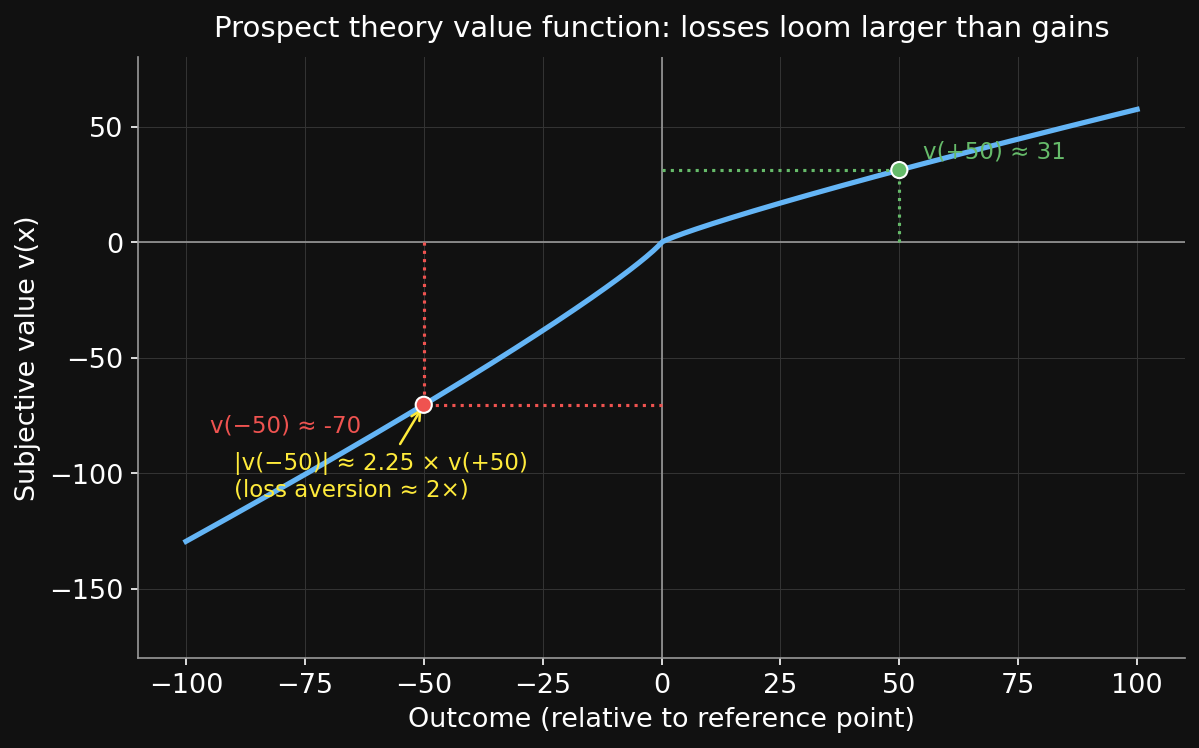
Loss aversion + the value function損失回避と価値関数

S-shape: concave for gains, convex + steeper for losses. Losses hurt ~2× more than equivalent gains feel good. Village link: “Loss aversion makes agents under-explore. Going to a new zone risks a bad day. Staying with your known zone feels safe even if EV of exploring is higher. The ε in ε-greedy forces exploration despite loss aversion — a normative override on a descriptive tendency.”

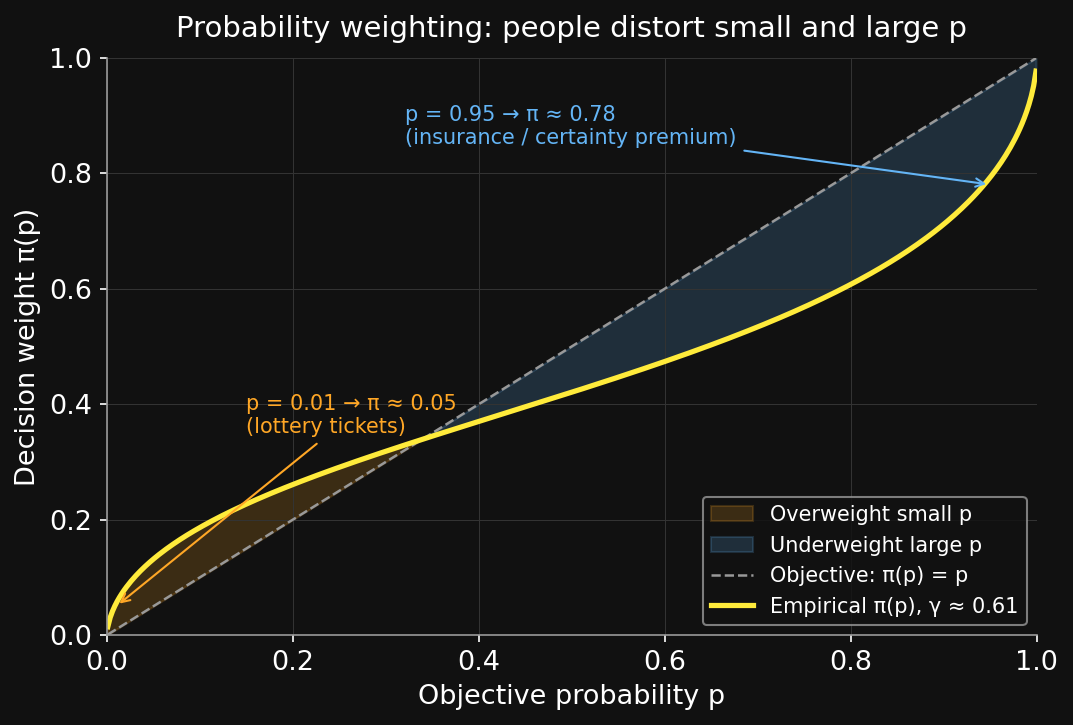
Probability weighting確率重みづけ

The decision-weight curve π(p) is inverted-S: bows above identity for small p, below identity for large p. Tied at π(0)=0, π(1)=1. Crossover around p ≈ 0.35.

The two effects map to different real-world phenomena — keep them straight:

• Small p overweighted → lottery tickets and buying insurance against rare disasters. You insure your house against fire (p ≈ 0.003) even though the premium has negative EV. Subjectively π(0.003) is bigger than 0.003, so the dread of fire feels heavier than its objective probability warrants. Same machinery as lottery tickets — overweighting tiny win probabilities. Both lottery and “insurance against rare loss” live on the small-p side.

• Large p underweighted → the certainty premium. Choose between (a) certain $3000 or (b) 80% chance of $4000. EU says take (b): EV = $3200. Most pick (a). Why? π(1.0) = 1 by definition, but π(0.8) < 0.8 — the gap between “definitely” and “very likely” feels bigger than the gap between “very likely” and “somewhat likely.” People pay a premium for certainty, not just for higher EV. This also shows up when you buy full coverage instead of 99% coverage: the last sliver of residual risk feels heavier than its objective π(0.997 → 1) jump.

Easy mnemonic: lottery + rare-disaster insurance both = small-p overweight. Certainty premium = large-p underweight. Insurance touches both sides but for different reasons (insuring against rare loss vs paying extra for the last 1% of coverage).

Prospect theory — the equationプロスペクト理論 — 式

Expected utility (the normative model):

EU(L) = \sum_i p_i \cdot u(x_i)

Prospect theory (the descriptive model):

V(L) = \sum_i \pi(p_i) \cdot v(x_i)

Same shape. Two substitutions: objective probability p → subjective weight \pi(p); objective value u(x) → subjective value v(x) relative to a reference point.

The claim: humans still aggregate probability × value — just not the probabilities and values you’d expect.

Kahneman won the 2002 Nobel Prize in Economics for this. (Tversky had died in 1996; the prize isn’t awarded posthumously.)

期待効用（規範モデル）：

EU(L) = \sum_i p_i \cdot u(x_i)

プロスペクト理論（記述モデル）：

V(L) = \sum_i \pi(p_i) \cdot v(x_i)

形は同じ。2つの置き換え：客観確率 p → 主観的重み \pi(p)；客観的価値 u(x) → 参照点に対する主観的価値 v(x)。

主張：人間はやはり確率×価値で集計する — ただし想定される確率や価値ではない。

カーネマンは2002年にノーベル経済学賞を受賞（トヴェルスキーは1996年に死去；ノーベル賞は死後には授与されない）。

~2 min. The pedagogical move: prospect theory is not a rejection of expected utility — it’s EU with two empirical substitutions. Same algebraic skeleton.

Walk through it on the board if there’s time: - “Expected utility says: multiply each outcome’s probability by its utility, sum up.” - “Prospect theory says: same operation, but probabilities go through a weighting function π first, and outcomes go through a value function v first.” - “The value function is the S-curve from the previous slide (loss-averse, reference-dependent). The π function is the curve from this one (small p overweighted, large p underweighted).”

The 2002 Nobel: Kahneman won the Sveriges Riksbank Prize in Economic Sciences in Memory of Alfred Nobel (the “Nobel in Economics”), shared with Vernon Smith. The citation specifically referenced integrating psychology into economics under uncertainty — prospect theory was the centerpiece. Tversky would have shared it but had died of melanoma in 1996.

Course-arc link: this is why Day 1 (normative Bayesian + EU) wasn’t wasted — prospect theory uses EU’s form. The empirical refinement is in the inputs. Same skeleton, different substance.

Source: Kahneman & Tversky (1979), “Prospect Theory: An Analysis of Decision under Risk.” Econometrica. Updated to “Cumulative Prospect Theory” by Tversky & Kahneman (1992) — the version where π operates on cumulative probabilities, fixing some axiomatic issues. Mention only if a student asks.

Closing the prospect-theory loopプロスペクト理論のまとめ

The picture from today so far:

   • Humans use heuristics — fast shortcuts that sometimes mislead.

   • Framing flips preferences. Losses hurt ~2× more than gains feel good.

   • Confirmation bias makes more data make things worse.

So what do we do?

Two options:

   1. Debias people — teach them, train them, ask them to be careful. Mostly doesn’t work (Lord/Lepper/Preston “be unbiased” intervention from earlier today).

   2. Redesign the choice environment. — meet people where they are. This is what nudging does — coming up after the break.

今日ここまでの全体像：

   • 人間はヒューリスティックを使う — 時に誤らせる速いショートカット。

   • フレーミングは選好を反転させる。損失は同等の利得よりも約2倍痛い。

   • 確証バイアスは、データが増えるほど状況を悪化させる。

ではどうするか？

2つの選択肢：

   1. 人をバイアス除去する — 教える、訓練する、慎重になるよう求める。ほとんど機能しない（今日の前半で扱ったLord/Lepper/Preston「公平に判断して」介入）。

   2. 選択環境を再設計する。— 人をありのまま受け入れる。これがナッジ — 休憩後に扱う。

~3 min. Prospect-theory closer + setup for nudging segment. Reframes the entire day’s worth of bias content as a problem statement, then teases the answer: nudging.

The “debias vs redesign” framing is the key pedagogical move. Students might assume the answer to bias is “teach people more” — but the confirmation-bias slides earlier in Day 2 showed that’s the failing intervention (Lord/Lepper/Preston 1984: “be unbiased” had basically no effect; “consider the opposite” worked because it forced System 2 engagement). The same logic generalizes: passive instruction doesn’t fix biases, but redesigning the choice architecture does.

This slide is intentionally shorter than the old “Course arc connection” because the organ-donor + MP4 framing now live in the dedicated Nudging segment after the break. Don’t repeat that material here — just tease “the answer is coming.”

Break — 10 minutes休憩 — 10分

10 min. After the break we shift from “what humans do wrong” (H&B + Prospect) to “what we can do about it” (Nudging).

Up next — Day 2 agenda次はここ — 第2日 アジェンダ

• Heuristics and biasesヒューリスティックとバイアス 0:00
• Prospect theoryプロスペクト理論 0:35
• Break休憩 0:55
• Nudging — choice architectureナッジ — 選択アーキテクチャ 1:05
• MP2 in-class workMP2 授業内作業時間 1:35
• MP2 guided discussionMP2 ガイド付き議論 2:28
• Three-week arc + Week 43週間の流れ + 第4週 2:48
• Buffer / Q&A予備 / Q&A 2:56

Nudging — choice architectureナッジ — 選択アーキテクチャ

30 min. Pivot point. Day 2 has shown bias after bias — now we ask: given these biases, what do we DO? Thaler & Sunstein’s answer: design the architecture people choose within, rather than trying to debias the people. Japan-framed throughout. Closes with the MP4 setup: fishing policy IS choice architecture.

There is no neutral menu中立的なメニューは存在しない

A school cafeteria has to put something first in the lunch line.

   • Pizza first → students grab pizza.

   • Salad first → students grab salad.

Someone has to decide what comes first.

The question is not “should we influence?” — that’s already happening, no matter what you do.

The question is “how should we influence?”

Thaler & Sunstein (2008): choice architecture is the way options are presented. Nudging = designing the architecture to steer choices toward better outcomes — without restricting them.

学校のカフェテリアは、ランチの列に何かを最初に置かなければならない。

   • ピザを最初に → 学生はピザを取る。

   • サラダを最初に → 学生はサラダを取る。

誰かが「何を最初に置くか」を決めなければならない。

問いは「影響を与えるべきか？」ではない — 何をしても影響は既に起きている。

問いは「どう影響を与えるべきか？」

Thaler & Sunstein (2008)：選択アーキテクチャとは選択肢の提示の仕方。ナッジは、選択を制限せずに、より良い結果へ向けるアーキテクチャの設計。

~4 min. The cafeteria example is the canonical opener from Thaler & Sunstein. The key move: “neutral” is impossible because the act of presentation already shapes choice. This dissolves the libertarian objection (“don’t influence me”) before it can land — you’re already being influenced; the only question is by what.

Japan-specific tie-in (verbal, not on slide): kyūshoku (school lunch) in Japan is already heavily designed. The point isn’t “Japan should start designing choices” — it already does, very deliberately. The question is whether other choice architectures (organ donation, retirement) get the same intentional design.

Source: PSYC414 Lec 13 slide 9 + Thaler & Sunstein 2008 Nudge.

What is a nudge?ナッジとは？

A nudge steers without restricting. You can still pick anything; the architecture just makes some choices easier.

Six families (Sunstein 2017):

   1. Just-in-time info — GPS reroutes; “you’ve had 800 cal today”

   2. Mandatory info — cigarette warnings; energy-efficiency labels

   3. Defaults & opt-in/opt-out — organ donor checkboxes; 401(k) auto-enroll

   4. Visual attention & effort — what’s at eye level; what’s two clicks away

   5. Social norms — “9 out of 10 hotel guests reuse towels”

   6. Active / forced choice — “you must select a retirement plan to continue”

We’ll look at three: defaults, the cafeteria, and active choice.

ナッジは制限せずに方向づける。何でも選べるけど、アーキテクチャによって特定の選択がやりやすくなる。

6つの分類（Sunstein 2017）：

   1. タイムリーな情報 — GPSの経路変更；「今日800kcal摂取した」

   2. 義務的情報 — タバコの警告；省エネ性能ラベル

   3. デフォルトとオプトイン/アウト — 臓器提供のチェック欄；401(k)自動加入

   4. 視覚的注意と労力 — 何が目の高さにあるか；何が2クリック先にあるか

   5. 社会規範 — 「ホテル客の10人中9人がタオルを再利用」

   6. 能動的/強制的選択 — 「次へ進むには年金プランを選択してください」

今日は3つ見る：デフォルト、カフェテリア、能動的選択。

~4 min. The six-family taxonomy from Sunstein 2017 (also in PSYC414 Lec 13). Don’t dwell on all six — give one example per type and move on. The takeaway is breadth: nudging is a family of techniques, not one trick. Pick three to go deep on (next 3 slides).

The “social norms” bullet is a deliberate setup: students may ask “what about misleading or manipulative norms?” — that’s the right question and leads naturally into the ethics conversation if you have time. If not, defer.

Defaults — organ donation, Japan vs Europeデフォルト — 臓器提供、日本 vs 欧州

Same people. Same preferences. Different forms.

Country	System	Donor rate
Austria, France, Spain, Belgium	opt-out	85–99%
Germany, UK (historical)	opt-in	~10–25%
Japan	opt-in (+ family veto)	~12%

Expressed-preference studies show similar populations have similar willingness to donate. The form did the deciding — not the values.

Why: filling forms is costly (default wins by inaction); defaults signal social norms; defaults relieve an emotionally hard decision.

同じ人々。同じ選好。異なる書式。

国	制度	提供率
オーストリア、フランス、スペイン、ベルギー	オプトアウト	85–99%
ドイツ、英国（過去）	オプトイン	~10–25%
日本	オプトイン（+家族拒否権）	~12%

表明された選好の調査では、各国の人々の提供したい気持ちは実は似ている。決めているのは書式、価値観ではない。

なぜ：書式記入はコストが高く、デフォルトは何もしないことで勝つ；デフォルトは社会規範を示す；感情的に難しい決定の負担を和らげる。

~6 min. This is the headline example. The Japan vs Europe comparison is visceral and the numbers are dramatic — 12% vs 99%. The point is NOT that opt-out is morally better than opt-in. The point is that the form is deciding for people, regardless of what their actual preferences are.

Japan-specific nuance: Japan’s family-veto provision compounds the opt-in default. Even when an individual has registered consent, the family can still refuse at the time of death. This is a second layer of friction. The 2010 law revision was supposed to increase rates by making opt-in easier; it had only modest effect because the friction was never the form complexity — it was the cultural framing of having to actively register.

Optional discussion: “Is opt-out coercive?” — Sunstein’s answer is no, because you can still opt out (it’s just one click). Compare to mandatory donation (which IS coercive). The libertarian-paternalism framing matters here.

Source: PSYC414 Lec 13 slide 23 + Johnson & Goldstein 2003.

Cafeteria layout — kyūshoku as choice architectureカフェテリア配置 — 給食という選択アーキテクチャ

The cafeteria experiment (Just & Wansink, 2009): Move fruit to the front, replace soda with water — keep fries available for those who want them.

   • 21% fewer calories per meal, 44% less fat, 43% less salt

Same children. Same prices. Same options. Different layout.

Japan already does this — at scale. Kyūshoku (給食) is a national nutrition program: balanced portions, no choice menus, eaten with the teacher. Japan’s school-age obesity rate is among the OECD’s lowest — kyūshoku is one cited reason.

The lesson: when you take design seriously, you use these effects deliberately. When you don’t, you get them anyway — without choosing the direction.

カフェテリア実験（Just & Wansink, 2009）：フライドポテトをフルーツに替えて列の前に、コーラを水に替える — ポテトはまだ取れる。

   • カロリー21%減、脂質44%減、塩分43%減

同じ子供たち。同じ価格。同じ選択肢。違うのは配置だけ。

日本はすでにこれを大規模にやっている。 給食は国家設計の栄養プログラム：バランスの取れた量、選択メニューなし、先生と一緒に食べる。日本の学齢期肥満率はOECD最低水準 — 給食はその理由の一つ。

教訓：設計を真剣に取り組めば、これらの効果を意図的に使える。取り組まなければ、効果は出るが、方向は選べない。

~5 min. The cafeteria study is the textbook positive-nudge example. The kyūshoku tie-in is the Japan-specific anchor: students live this every school day until middle school. They’ve been inside an intentional choice architecture without naming it.

If asked “what about freedom of choice in school lunch?” — note that Japan’s kyūshoku is highly defensible BECAUSE it’s nationally designed and transparent, not because it removes choice. Compare to US-style cafeterias where the “free choice” framing hides the fact that someone’s still deciding what’s available.

Source: PSYC414 Lec 13 slide 13 (calorie/fat/salt numbers) + Just & Wansink 2009.

Retirement defaults — the iDeCo gap退職金デフォルト — iDeCoの隔たり

Madrian & Shea (2001) — US retirement plans:

System	After 3 months	After 3 years
Opt-in (active enrollment required)	20%	65%
Opt-out (automatic enrollment)	90%	98%

Same employees. Same plan. Same incentive. The default carries ~70 percentage points.

Japan’s iDeCo: strong tax incentives, available to nearly all working adults since 2017. Actual participation: ~3%. The friction is active choice — strong incentives lose to do-nothing.

Could we just educate people instead? Duflo & Saez (2003): randomized info intervention → ~1pp. Defaults → ~70pp. Education is the first instinct; rarely the working one.

Madrian & Shea (2001) — 米国の年金プラン：

制度	3ヶ月後	3年後
オプトイン（能動的加入が必要）	20%	65%
オプトアウト（自動加入）	90%	98%

同じ従業員。同じプラン。同じインセンティブ。デフォルトが約70パーセンテージポイントを動かす。

日本のiDeCo：強い税制優遇、2017年以降ほぼ全ての勤労者が利用可能。実際の加入率：約3%。 摩擦は能動的選択 — 強いインセンティブでも何もしないに負ける。

ただ教育すれば？ Duflo & Saez (2003)：無作為化情報介入は約1pp、デフォルトは約70pp。教育は最初の直感だが、ほぼ機能しない。

~5 min. The iDeCo example is high-stakes for Japanese students — retirement adequacy is a national-level discussion in Japan, and most undergrads will have iDeCo eligibility within a year of graduation but will not enroll.

The point is NOT that Japan should automatically enroll everyone in iDeCo (legal/political complications). The point is that the current policy reveals exactly the gap nudge theory predicts: strong incentive + active-choice requirement = low uptake.

The 70-percentage-point default effect from Madrian & Shea is the canonical retirement-defaults result. It’s been replicated many times since.

Education-doesn’t-work contrast. The Duflo & Saez 2003 line is the natural complement: same outcome (retirement enrollment), opposite intervention (information seminar instead of default change), opposite-magnitude effect (~1pp vs ~70pp). It also generalizes — financial-literacy interventions across many domains (savings, debt, investing) consistently produce small-to-null behavioral effects (see Fernandes/Lynch/Netemeyer 2014 meta-analysis if pressed). This parallels the Day-2-earlier “be unbiased” finding: passive instruction doesn’t move behavior, structural change does. Two flavors of the same lesson.

Optional question if time: “Is automatic enrollment paternalistic?” Yes — and the question is whether libertarian paternalism (you can still opt out, freely, easily) is okay when the alternative is de facto paternalism by inaction (the system as-is is also forcing an outcome on people).

Source: PSYC414 Lec 13 slide 24 + Madrian & Shea 2001 + Duflo & Saez 2003 (QJE) + JILPT iDeCo statistics.

Be your own choice architect自分の選択アーキテクトになる

You learned about these biases in others. They operate on you too. Some applied advice from today’s lecture:

   • Automate the things you’d procrastinate on. Set up automatic transfers to savings/investments on payday. Removes the daily choice point where present-bias wins.

   • Pick a low-cost index fund and don’t touch it. Active funds underperform on average — you’d know that if availability weren’t biasing you toward the success stories you’ve heard about.

   • Don’t check your portfolio daily. Loss aversion makes daily fluctuations hurt 2× more than they help. Monthly is plenty; annual is fine.

   • Sleep on big purchases. System 2 needs time. The thing you “definitely” want at midnight is rarely the thing you want a week later.

Choice architecture is not just for governments. You can build it for yourself.

今日の講義で他人のバイアスを学んだ。それは皆さん自身にも働く。今日の内容を自分の生活に活かす：

   • 先延ばしにしてしまうことは自動化する。給料日に貯蓄・投資への自動振込を設定。現在バイアスが勝つ日々の選択点を取り除く。

   • 低コストのインデックスファンドを選び、触らない。アクティブ運用は平均すれば指数に負ける — 利用可能性バイアスが成功例ばかりを目立たせていなければ気付くはず。

   • ポートフォリオを毎日チェックしない。損失回避により、日々の変動は嬉しさの2倍痛い。月次で十分、年次でも問題ない。

   • 大きな買い物は一晩寝かせる。システム2には時間が必要。深夜に「絶対欲しい」物は、一週間後にはほぼ欲しくない。

選択アーキテクチャは政府だけのものではない。自分自身のために設計できる。

~3 min. Closing applied move: take everything today and apply it to your own decisions. The segment has been about policy choice architecture (organ donation, retirement, cafeteria); this slide shifts to personal choice architecture.

Japan-specific concrete handles (mention live, don’t put on the slide — vehicles change, and slides screenshot):

• Automating saving: 自動振込 on payday into a separate savings account or directly into NISA/iDeCo. Removes the monthly “should I save this month?” choice point.
• NISA vs iDeCo: NISA (especially the new 2024 expanded version, つみたて投資枠) is the friendlier default — flexible, accessible. iDeCo locks money until 60 but has stronger tax advantages. For most students, “open a NISA, set up auto-buy into an all-country index fund (eMAXIS Slim 全世界株式 or similar), don’t touch it” is the advice.
• Active vs index: SPIVA reports consistently show >80% of actively-managed funds underperform their benchmark over 10+ years. The same pattern holds for Japan-domiciled funds. Availability bias is the mechanism: you hear about the winners, not the losers.
• Loss aversion + checking frequency: Benartzi & Thaler (1995) “myopic loss aversion” — investors who check frequently take less risk and earn less long-term, because day-by-day red dominates their experience.
• Sleep on it: matches the “consider the opposite” intervention from Day 2’s confirmation-bias slide. Same System-2 engagement move, applied to consumer decisions.

Cultural caveat for the room: Japanese cultural framing around money/investing is more risk-averse than US baseline (decades of deflation, post-bubble caution). Don’t push aggressively; present the advice as “if you decide to invest, here’s how to avoid the predictable mistakes,” not “you should invest.” The deeper point is that the biases are universal even when financial vehicles differ.

Pedagogical close: this slide takes a course about agents and turns it inward — students are agents too, and the same design tools work on the self. Sets up the “you’re not just a user of these systems, you’re a designer” framing that will recur in MP4 + Week 4 (multi-agent dynamics).

If short on time, this slide can be cut entirely; the iDeCo slide already lands the segment’s central point. Keep it if energy is high enough for the inward turn.

Up next — Day 2 agenda次はここ — 第2日 アジェンダ

• Heuristics and biasesヒューリスティックとバイアス 0:00
• Prospect theoryプロスペクト理論 0:35
• Break休憩 0:55
• Nudging — choice architectureナッジ — 選択アーキテクチャ 1:05
• MP2 in-class workMP2 授業内作業時間 1:35
• MP2 guided discussionMP2 ガイド付き議論 2:28
• Three-week arc + Week 43週間の流れ + 第4週 2:48
• Buffer / Q&A予備 / Q&A 2:56

MP2 in-class workMP2 授業内作業時間

53 min. Students work on MP2 individually. Joe + Ira circulate, answer questions, push students to articulate WHY a bug is wrong (normative principle) rather than just patching syntax.

Key things to listen for and challenge: - “AI told me to change this” → “but WHY is that wrong? what should the agent do here?” - “I made it work” → “what ‘working’ means matters. Show me the belief trajectory.” - “I haven’t found any bugs yet” → “have you traced one update by hand from a non-50 starting belief?”

The 53 min replaces the long-form presentations from the original plan. Students get more debugging time and the discussion that follows is grounded in fresh work, not stale memory of work-from-home.

Work it through作業時間

~50 minutes. Continue debugging MP2.

   • Use AI freely. But you must be able to explain WHY each bug is wrong — not just that AI flagged it.

   • Trace at least one belief update by hand before trusting AI’s read.

   • Talk to a neighbor when you find something interesting — but the debugging is yours.

Joe and Ira will circulate. Flag us if you’re stuck — but try the opposite question first (“if AI’s fix were wrong, how would I know?”).

We’ll regroup in ~50 min for a guided discussion of what you found.

約50分。MP2のデバッグを続ける。

   • AIは自由に使ってよい。ただし、各バグがなぜ間違いかを説明できなければならない — AIが指摘したからではなく。

   • AIの読解を信頼する前に、少なくとも1つの信念更新を手計算でたどる。

   • 何か面白いことを見つけたら隣の人と話してよい — でもデバッグは自分の仕事。

ジョー先生とアイラ先生が巡回する。詰まったら声をかけて — でもまず逆の問いを試して（「AIの修正が間違いだったら、どう気づくか？」）。

約50分後にガイド付き議論で集合 — 何を見つけたかを共有。

Sets ground rules and reminds students of the AI-collaboration discipline from Day 1’s Consider-the-Opposite slide. The “trace one update by hand” instruction is critical — it’s the inoculation against confirmation bias when reading AI’s output.

With 5 students, pair-work is awkward; everyone debugs their own copy. Side-by-side conversation is welcome when something interesting comes up, but the debugging itself is individual. Joe + Ira circulate so the support is teacher-led, not peer-led.

Up next — Day 2 agenda次はここ — 第2日 アジェンダ

• Heuristics and biasesヒューリスティックとバイアス 0:00
• Prospect theoryプロスペクト理論 0:35
• Break休憩 0:55
• Nudging — choice architectureナッジ — 選択アーキテクチャ 1:05
• MP2 in-class workMP2 授業内作業時間 1:35
• MP2 guided discussionMP2 ガイド付き議論 2:28
• Three-week arc + Week 43週間の流れ + 第4週 2:48
• Buffer / Q&A予備 / Q&A 2:56

MP2 guided discussionMP2 ガイド付き議論

20 min. Bug-driven group conversation, NOT formal presentations. Joe drives with open prompts, students contribute findings in turn. Joe synthesizes on the board (whiteboard or shared doc).

Goal: surface the pattern — which bug families AI catches vs misses, what kind of understanding is doing the work when humans catch things AI doesn’t. This pattern is the takeaway: the System-2 / Consider-the-Opposite discipline from earlier today is concretely useful for AI-collaboration debugging.

Time budget within 20 min: - 5 min — quick round, each student names ONE bug + how they caught it - 10 min — Joe-led discussion of the hardest bug (whichever the group says was hardest) - 5 min — synthesis: “what kinds of bugs is AI good/bad at?” — students propose categories

Group conversationグループ討論

Each of you, one bug:

   • What was it?

   • How did you notice?

   • Did AI help, hurt, or miss?

Then we’ll talk together about the hardest bug — what did it take to catch?

Closing question — propose a pattern:

*“AI is good at catching . AI is bad at catching . The reason is ___.”*

一人ずつ、バグ1つ：

   • 何だった？

   • どう気づいた？

   • AIは助けた？妨げた？見逃した？

次にグループで最も難しかったバグについて話す — 何があれば気づけたか？

締めの問い — パターンを提案する：

*「AIは_を見つけるのが得意。AIは_を見逃しがち。理由は___。」*

The “closing question” template scaffolds the synthesis. Likely answers students will converge on:

• AI catches: syntax bugs, off-by-one errors, type errors, anything where the bug shows up in the error message or in obviously-broken output.
• AI misses: conceptual bugs where the code RUNS but does the wrong thing, especially when the “wrong thing” looks plausible (like α=1.0 making the belief = latest observation).
• The reason: AI evaluates code by form-matching to patterns it’s seen. Conceptual bugs preserve form but break meaning. Humans catch them when they have a normative model of what the code SHOULD do (e.g., “EMA should converge, not blow up”).

This is the System-2 win condition from Day 1 wrapped up. Tie it back: “Day 1 we said your MP1 intuition is your most powerful debugging tool. Today you have evidence.”

If discussion has good energy, let it run; cap at 20 min hard so nudging-arc-wrap have their time.

Up next — Day 2 agenda次はここ — 第2日 アジェンダ

• Heuristics and biasesヒューリスティックとバイアス 0:00
• Prospect theoryプロスペクト理論 0:35
• Break休憩 0:55
• Nudging — choice architectureナッジ — 選択アーキテクチャ 1:05
• MP2 in-class workMP2 授業内作業時間 1:35
• MP2 guided discussionMP2 ガイド付き議論 2:28
• Three-week arc + Week 43週間の流れ + 第4週 2:48
• Buffer / Q&A予備 / Q&A 2:56

Three-week arc3週間の流れ

15 min synthesis + Week 4 preview.

Where we’ve beenこれまでの流れ

Week 1 — Why should we care?

Plurality: technology and democracy are drifting apart. The path forward isn’t centralized AI or atomized markets — it’s digital democracy, technology that strengthens diverse social connections.

Week 2 — How do agents perceive?

Through their Umwelt — the noisy, partial slice of the world a particular agent can sense. Marr’s levels (computation / algorithm / implementation) let us analyze the same agent at different scales.

Week 3 — How do agents reason and decide?

   • Normatively: Bayes + expected utility

   • Descriptively: heuristics, biases, prospect theory

   • The gap is where design lives.

第1週 — なぜ気にするのか？

Plurality：テクノロジーと民主主義が乖離している。進むべき道は中央集権的AIでも分断された市場でもなく、デジタル民主主義 — 多様な社会的繋がりを強めるテクノロジー。

第2週 — エージェントはどう知覚するのか？

環世界（Umwelt）を通して — エージェントが感知できる、ノイズが多く部分的な世界の一部分。Marrのレベル（計算・アルゴリズム・実装）で同じエージェントを異なる粒度で分析できる。

第3週 — エージェントはどう推論・決定するのか？

   • 規範的には：ベイズ + 期待効用

   • 記述的には：ヒューリスティック、バイアス、プロスペクト理論

   • ギャップこそ設計の住処。

Synthesis. Make the arc visible. ~3-4 min.

Each week now has a one-sentence gloss in dim text — students three weeks out from Week 1 may not remember what “Plurality” or “Umwelt” specifically meant, and re-grounding them here makes the arc statement land. Don’t read the gloss aloud verbatim — it’s there as the visual anchor while you give a richer verbal recap from memory.

If asked to elaborate on the Week 1 gloss: Plurality (Weyl, Tang) argues against both Synthetic Technocracy (centralized AI control) and Corporate Libertarianism (atomized crypto-libertarianism), proposing instead that the path forward is technology that strengthens diverse decentralized social connections — what they call “Digital Democracy.”

If asked about Umwelt: from von Uexküll’s biology — every organism inhabits its own perceptual world made of the signals it can sense and act on. A tick’s Umwelt has butyric acid and warmth; a fish’s Umwelt has water pressure gradients. MP1’s fishing agents have the zone observation Umwelt, no more.

Where we’re going — Week 4 & beyond次週：第4週と以降

Week 4: multi-agent dynamics.

What happens when agents interact?

   • Multiple agents, shared resources (the fishing village + its neighbors)

   • Tragedy of the commons

   • Coordination, signaling, trust

“How do I decide?” becomes “what happens when we ALL decide?”

MP4 — fishing policy as choice architecture. You’ll design the rules: defaults, framing, norms. Today’s nudging segment was the toolkit. MP4 is the application.

第4週：マルチエージェント動学。

エージェントが相互作用すると何が起こるか？

   • 複数エージェント、共有資源（漁村と隣接する村）

   • コモンズの悲劇

   • 協調、シグナリング、信頼

「私はどう決めるか」が「皆で決めるとどうなるか」に変わる。

MP4 — 選択アーキテクチャとしての漁業政策。ルールを設計する：デフォルト、フレーミング、規範。今日のナッジングがツールキット。MP4が応用編。

Hand-off slide. ~3 min. The MP4 framing now leans on the nudging segment students just heard — choice architecture isn’t introduced here for the first time. Reuse the vocabulary; don’t re-define.

If a student asks “what’s the assignment?”: MP4 is a policy-design exercise. Given a population of agents with known biases (from this week) and known interaction dynamics (from Week 4 content), design fishing-policy choice architecture: what’s the default rule, what frame is used, what norm signal is broadcast, how does it scale across agents? Multiple proposals, simulated together, compare outcomes.

Don’t promise specifics on MP4 here — keep it directional. Joe will detail MP4 at the start of Week 4 itself.

Buffer / Q&A予備 / Q&A

10 min. Open floor.